One of the long term aims of the weather station is to take the system off grid. This will mean using an alternative energy source, something other than mains electricity. This usually means using solar energy to charge batteries in order to keep the system running.
Another scenario that will need to be considered is the case where the weather station is collecting data but is unable to connect to the internet. In this case it is desirable for the weather station to continue to collect data, record the date and time the observation was made and also store the readings. The system can then upload the data when the network connection is once available once more.
This article presents a possible solution to one problem and a possible solution to another:
- Reducing power by putting the system to sleep
- Recording the date / time when the system is not connected to the Internet
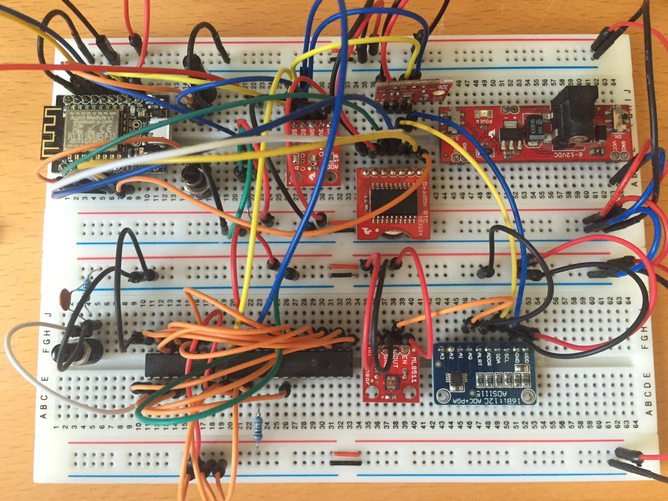
The solution being considered is a Real Time Clock (RTC) module based upon the DS3234 chip.
DS3234 RTC
The DS3234 is a real time clock module with a built in temperature controlled oscillator. It is a relatively self-contained module requiring few external components. The chip is programmed over the built in SPI interface.
A summary of the important features being considered are:
- Built in alarm(s)
- Battery back up
- Built in oscillator
- Interrupt on alarm
One additional feature that may be useful is the provision of 256 bytes of battery backed up RAM.
The interrupt generated by the alarms can be used to trigger the Oak to take action. In this way it may be possible for the Oak to sleep for a period of time waiting for a signal from the RTC. The RTC will run in much lower power mode than the Oak.
One disadvantage of this module, at the time of writing, was the lack of code that would either provide the functioality required or work reliably on the Oak.
Time to break out the C++ compiler.
Controlling the DS3234
Before we look at the software, it is worth spending a little time to review how the DS3234 is controlled. The RTC chip uses write operations to a series of registers in order to control the functionality of the chip. The register map is as follows:
| Register Read Address | Contents |
| 0x00 | Current time seconds |
| 0x01 | Current time minutes |
| 0x02 | Current time hour |
| 0x03 | Current time day |
| 0x04 | Current time date |
| 0x05 | Current time month |
| 0x06 | Current time year |
| 0x07 | Alarm 1 seconds |
| 0x08 | Alarm 1 minutes |
| 0x09 | Alarm 1 hour |
| 0x0a | Alarm 1 day/date |
| 0x0b | Alarm 2 minutes |
| 0x0c | Alarm 2 hour |
| 0x0d | Alarm 2 day/date |
| 0x0e | Control register |
| 0x0f | Control / status register |
| 0x10 | Crystal aging offset |
| 0x11 | Temperature (MSB) |
| 0x12 | Temperature (LSB) |
| 0x13 | Disable temperature conversions |
| 0x14 | Reserved |
| 0x15 | Reserved |
| 0x16 | Reserved |
| 0x17 | Reserved |
| 0x18 | SRAM address |
| 0x19 | SRAM data |
Applications can write to the registers by setting bit 7 (i.e. add 0x80) in the address.
The register address is automatically incremented after a read or write operation. So to write the current time into the hours, minutes and seconds registers an application would simply write four bytes to the SPI bus; namely address 0x80 (write address for the seconds register) followed by the seconds, minutes and hour values.
The bit fields for the above registers are well defined in the DS3234 datasheet and are not covered in too much detail here and you are encouraged to download the datasheet for reference.
DS3234 Software – Private Interface
The full source code for this module can be downloaded from at the end of this article, the discussion about the software and it’s functionality will concentrate on the class definition in the header file. Those interested in the detail can jump into the source code at the end of the article.
So let’s have a look at the full header file:
#ifndef _DS3234_h
#define _DS3234_h

#include <BitBang\BitBang.h>

#if defined(ARDUINO) && ARDUINO >= 100
	#include "arduino.h"
#else
	#include "WProgram.h"
#endif

#define MAX_BUFFER_SIZE     256

//
//  Time structure.
//
struct ts
{
    uint8_t seconds;    // Number of seconds, 0-59
    uint8_t minutes;    // Number of minutes, 0-59
    uint8_t hour;       // Number of hours, 0-23
    uint8_t day;        // Day of the month, 1-31
    uint8_t month;      // Month of the year, 1-12
    uint16_t year;      // Year >= 1900
    uint8_t wday;       // Day of the week, 1-7
};

//
//  Define the methods required to communicate with the DS3234 Real Tiem Clock.
//
class DS3234RealTimeClock
{
    public:
        //
        //  Enums.
        //
        enum Alarm { Alarm1, Alarm2, Both, Unknown };
        enum AlarmType { OncePerSecond, WhenSecondsMatch, WhenMinutesSecondsMatch,  // Alarm 1 options.
                         WhenHoursMinutesSecondsMatch, WhenDateHoursMinutesSecondsMatch, WhenDayHoursMinutesSecondsMatch,
                         OncePerMinute, WhenMinutesMatch, WhenHoursMinutesMatch,    // Alarm 2 options.
                         WhenDateHoursMinutesMatch, WhenDayHoursMinutesMatch };
        enum ControlRegisterBits { A1IE = 0x01, A2IE = 0x02, INTCON = 0x04, RS1 = 0x08, RS2 = 0x10, Conv = 0x20, BBSQW = 0x40, NotEOSC = 0x80 };
        enum StatusRegisterBits { A1F = 0x02, A2F = 0x02, BSY = 0x04, EN32Khz = 0x08, Crate0 = 0x10, Crate1 = 0x20, BB32kHz = 0x40, OSF = 0x80 };
        enum RateSelect { OneHz = 0, OnekHz = 1, FourkHz = 2, EightkHz = 3 };
        enum Registers { ReadAlarm1 = 0x07, WriteAlarm1 = 0x87,
                         ReadAlarm2 = 0x0b, WriteAlarm2 = 0x8b,
                         ReadControl = 0x0e, WriteControl = 0x8e,
                         ReadControlStatus = 0x0f, WriteControlStatus = 0x8f,
                         ReadAgingOffset = 0x10, WriteAgingOffset = 0x90,
                         ReadSRAMAddress = 0x18, WriteSRAMAddress = 0x98,
                         ReadSRAMData = 0x19, WriteSRAMData = 0x99 };
        enum DayOfWeek { Sunday = 1, Monday, Tuesday, Wednesday, Thursday, Friday, Saturday };
        //
        //  Construction and destruction.
        //
        DS3234RealTimeClock(const uint8_t);
        DS3234RealTimeClock(const uint8_t, const uint8_t, const uint8_t, const uint8_t);
        ~DS3234RealTimeClock();
        //
        //  Methods.
        //
        uint8_t GetAgingOffset();
        void SetAgingOffset(uint8_t);
        float GetTemperature();
        uint8_t GetControlStatusRegister();
        void SetControlStatusRegister(uint8_t);
        uint8_t GetControlRegister();
        void SetControlRegister(uint8_t);
        ts *GetDateTime();
        Alarm WhichAlarm();
        void SetDateTime(ts *);
        String DateTimeString(ts *);
        void SetAlarm(Alarm, ts *, AlarmType);
        void InterruptHandler();
        void ClearInterrupt(Alarm);
        void EnableDisableAlarm(Alarm, bool);
        void WriteToSRAM(uint8_t, uint8_t);
        uint8_t ReadFromSRAM(uint8_t);
        void ReadAllRegisters();
        void DumpRegisters(const uint8_t *);
        void ReadSRAM();
        void DumpSRAM();

    private:
        //
        //  Constants.
        //
        static const int REGISTER_SIZE = 0x14;
        static const int DATE_TIME_REGISTERS_SIZE = 0x07;
        static const int MEMORY_SIZE = 0xff;
        //
        //  Variables
        //
        int m_ChipSelect = -1;
        int m_MOSI = -1;
        int m_MISO = -1;
        int m_Clock = -1;
        uint8_t m_Registers[REGISTER_SIZE];
        uint8_t m_SRAM[MEMORY_SIZE];
        BitBang *m_Port;
        //
        //  Make the default constructor private so it cannot be called explicitly.
        //
        DS3234RealTimeClock();
        //
        //  Methods.
        //
        void Initialise(const uint8_t, const uint8_t, const uint8_t, const uint8_t);
        void SetRegisterValue(const Registers, uint8_t);
        uint8_t GetRegisterValue(const Registers);
        uint8_t ConvertUint8ToBCD(const uint8_t);
        void BurstTransfer(uint8_t *, uint8_t);
        void BurstTransfer(uint8_t *, uint8_t *, uint8_t);
        uint8_t ConvertBCDToUint8(const uint8_t);
};

#endif
Perversely, this discussion will start with the private data items and methods as these underpin the way in which the class provides the higher-level functionality.
Constants
The three constants define the size of the various register and RAM space within the chip.
REGISTER_SIZE
Defines the total number of bytes in the register bank excluding the reserved and SRAM registers.
DATE_TIME_REGISTERS_SIZE
Number of bytes holding the current date and time information.
MEMORY_SIZE
Number of bytes of SRAM.
Private Member Variables
The private member variables hold the state information for the class.
As noted in the datasheet for the DS3234, communication with the DS3234 is over the SPI bus. The first version of this class uses a software SPI class BitBang to provide this functionality.
m_Clock, m_MOSI, m_MISO, m_ChipSelect
The software SPI class allows the user to change the pins that provide the MOSI, MISO and Clock input/outputs. These four member variables record the pins used to provide the soft SPI bus.
m_Port
Instance of the class providing the SPI service.
m_Registers
Internal copy of the registers (up to the reserved registers).
m_SRAM
Internal copy of the SRAM.
Methods
The private methods provide the low level functionality supporting the public methods. These methods provide functions such as initialisation, communication and data conversion.
DS3234RealTimeClock()
The default constructor is made private to ensure that the developer cannot call this accidentally, forcing the use of the constructors that define the properties of the soft SPI bus.
void Initialise(const uint8_t chipSelect, const uint8_t mosi, const uint8_t miso, const uint8_t clock)
The four parameters inform the class which pins are used for the MOSI, MISO, Clock and Chip Select functions.
uint8_t ConvertBCDToUint8(const uint8_t value)
The values in the registers recording the date / time hold BCD values. This method provides a way to convert the DS3234 BCD values into a more natual (for the developer) uint8_t value.
uint8_t ConvertUint8ToBCD(const uint8_t value)
As noted above (see ConvertBCDToUint8), the DS3234 uses BCD to hold time vales. This methods provdes a method to convert uint8_t values to BCD before they are written to the registers.
uint8_t GetRegisterValue(const Registers reg)
Read a value from the specified register.
void SetRegisterValue(const Registers reg, const uint8_t value)
Set the specified register reg to value.
void BurstTransfer(uint8_t *dataToChip, uint8_t size) and void BurstTransfer(uint8_t *dataToChip, uint8_t *dataFromChip, uint8_t size)
As noted in the hardware discussion, the DS3234 will automatically increment the “address register” if multiple bytes of data are written to the SPI bus. These two methods take advantage of this functionality.
The first variant of the overloaded method, BurstTransfer(uint8_t *dataToChip, uint8_t size), transfers a number of bytes defined by size to the SPI bus. No data is read from the bus.
The second method,
BurstTransfer(uint8_t *dataToChip, uint8_t *dataFromChip, uint8_t size), both writes and reads
size bytes to/from the SPI bus.
In both cases, the first byte of the dataToChip buffer is set to the address of the first register to be read/written.
DS3234 Software – Public Interface
The public interface is the useful part of this class as it provides the functionality that is usable by the application developer.
Enumerated Types
The first group of items in the public interface are a series of enumerated types. These allow a meaningful name to be given to the various registers, bits within the registers and method parameters.
Alarm
There are two alarms on the DS3234, Alarm1 and Alarm2. These have slightly different capabilities as defined in the next enum.
enum Alarm { Alarm1, Alarm2, Both, Unknown };
This enum is also used to represent the type of alarm that has been generated.
AlarmType
The AlarmType represents the type of alarm being set. These have been put into two groups, one for each of the alarms:
enum AlarmType { OncePerSecond, WhenSecondsMatch, WhenMinutesSecondsMatch,  // Alarm 1 options.
                 WhenHoursMinutesSecondsMatch, WhenDateHoursMinutesSecondsMatch, WhenDayHoursMinutesSecondsMatch,
                 OncePerMinute, WhenMinutesMatch, WhenHoursMinutesMatch,    // Alarm 2 options.
                 WhenDateHoursMinutesMatch, WhenDayHoursMinutesMatch };
The first two lines represent the type of alarms that can be set on Alarm1, the second two lines can be used with Alarm2.
ControlRegisterBits
The values in this enum are the flags in the control register:
enum ControlRegisterBits { A1IE = 0x01, A2IE = 0x02, INTCON = 0x04, RS1 = 0x08, RS2 = 0x10, Conv = 0x20, BBSQW = 0x40, NotEOSC = 0x80 };
Two or more options can be set by or-ing the flags.
StatusRegisterBits
The status register as actually a combination of a number of bits that indicate the status of the DS3234 as well as some that control the action of the DS3234.
enum StatusRegisterBits { A1F = 0x02, A2F = 0x02, BSY = 0x04, EN32Khz = 0x08, Crate0 = 0x10, Crate1 = 0x20, BB32kHz = 0x40, OSF = 0x80 };
RateSelect
It is possible to generate a square wave at one of four frequencies on the interrupt pin. These flags determine the frequency of the generated signal:
enum RateSelect { OneHz = 0, OnekHz = 1, FourkHz = 2, EightkHz = 3 };
Registers
There are a total of 25 register addresses on the DS3234, containing information about the time, alarms and various other functions of the DS3234. This enumeration contains the addresses of several of the registers excluding the time register addresses:
enum Registers { ReadAlarm1 = 0x07, WriteAlarm1 = 0x87,
                 ReadAlarm2 = 0x0b, WriteAlarm2 = 0x8b,
                 ReadControl = 0x0e, WriteControl = 0x8e,
                 ReadControlStatus = 0x0f, WriteControlStatus = 0x8f,
                 ReadAgingOffset = 0x10, WriteAgingOffset = 0x90,
                 ReadSRAMAddress = 0x18, WriteSRAMAddress = 0x98,
                 ReadSRAMData = 0x19, WriteSRAMData = 0x99 };
The current time register addresses have been excluded as there are methods available to set and get the time using the ts structure.
DayOfWeek
The day of the week is represented by a number inthe range 1 to 7. The actual day represented is arbitary and Sunday has been selected for the number 1:
enum DayOfWeek { Sunday = 1, Monday, Tuesday, Wednesday, Thursday, Friday, Saturday };
Constructor and Destructor
As already noted, the default constructor has been made private but two public constructors have been created. This ensures that the developer is forced to define one or more of the parameters for the SPI bus.
DS3234RealTimeClock(const uint8_t chipSelect)
The only parameter to this constructor is the pin to be used for chip select.
If this constructor is used the default pins are used for MOSI, MISO and SCLK.
DS3234RealTimeClock(const uint8_t chipSelect, const uint8_t mosi, const uint8_t miso, const uint8_t clock)
Using this method, the developer can override all of the pins used for the SPI bus.
~DS3234RealTimeClock()
Destructor to release all of the resources held by the instance of the class.
Methods
All of the high level functionality of the class is exposed by the public methods.
uint8_t GetAgingOffset() & SetAgingOffset(uint8_t agingOffset)
Get or set the value for the aging offset register. This is the value used to apply to the oscillator to compensate for variations in temperature.
float GetTemperature()
Get the current temperature.
uint8_t GetControlStatusRegister()
Get the current contents of the control register.
void SetControlRegister(const uint8_t controlRegister)
Set the control register to the specified value. The ControlRegisterBits can be or-ed together to build up the required value.
ts *GetDateTime()
Get the current date and time.
void SetDateTime(ts *dateTime)
Set the current date and time to the specified value.
String DateTimeString(ts *theTime)
Convert theDate into a string using the format dd-mon-yyyy hh-min-ss.
void SetAlarm(Alarm alarm, ts *time, AlarmType type)
Set the alarm time to time and the type of the alarm type to type.
void EnableDisableAlarm(Alarm alarm, bool enableOrDisable)
Turn the specified alarm on (if enableOrDisable is true) or off (if enableOrDisable is false).
void ClearInterrupt(Alarm alarm)
Clear the interrupt flag for the specified alarm. If both interrupt have been triggered then the application will need to clear both alarms in order to reset the interrupt line on the DS3234.
Alarm WhichAlarm()
Determine which alarm has generated the interrupt.
void InterruptHandler()
This method has been provided to allow the application to call a generic interrupt handler. This method is not currently implemented.
SRAM Methods
There are 256 bytes of battery backed up SRAM in the DS3234 and the following two methods expose this memory to the developer.
void WriteToSRAM(uint8_t address, uint8_t data)
Write a byte of data into the specified address in the battery backed up SRAM.
uint8_t ReadFromSRAM(uint8_t)
Read the byte of data at the specified address in the battery backed up SRAM.
Diagnostic Methods
The following methods are used for diagnostic purposes.
void ReadAllRegisters()
Read the contents of the entire register set within the DS3234 and place them in the internal private variable m_Registers variable.
void DumpRegisters(const uint8_t *)
Dump the regsiters to the serial port. The ReadAllRegisters should be called before calling this method.
void ReadSRAM()
Read the content of the SRAM and store this in the private internal m_SRAM variable.
void DumpSRAM()
Display the contents of the battery backed up SRAM to the serial port.
Example application
Several example applications were developed throughout the development of the library. The application below illustrates several of the key features of the library.
First thing that is needed is an instance of the DS3234 class:
DS3234RealTimeClock *rtc = new DS3234RealTimeClock(6);
Next up, we need to setup the DS3234 and attach an interrupt handler.
void setup()
{
    ts *dateTime;

    Serial.begin(9600);
    Serial.println("Setup in progress.");
    rtc->SetControlRegister(DS3234RealTimeClock::INTCON);
    rtc->ClearInterrupt(DS3234RealTimeClock::Alarm1);
    rtc->ClearInterrupt(DS3234RealTimeClock::Alarm2);

    //dateTime = new (ts);
    //dateTime->day = 27;
    //dateTime->wday = 5;
    //dateTime->month = 5;
    //dateTime->year = 2016;
    //dateTime->minutes = 05;
    //dateTime->hour = 13;
    //dateTime->seconds = 0;
    //rtc->SetDateTime(dateTime);

    dateTime = rtc->GetDateTime();
    dateTime->minutes += 2;
    if (dateTime->minutes >= 60)
    {
        dateTime->minutes -= 60;
    }
    dateTime->seconds = 0;
    Serial.print("Setting alarm for ");
    Serial.println(rtc->DateTimeString(dateTime));
    rtc->SetAlarm(DS3234RealTimeClock::Alarm1, dateTime, DS3234RealTimeClock::WhenMinutesSecondsMatch);
    rtc->EnableDisableAlarm(DS3234RealTimeClock::Alarm1, true);
    pinMode(5, INPUT_PULLUP);
    attachInterrupt(5, RTCInterrupt, FALLING);
    Serial.println("Setup complete.");
}
setup‘s first job is to clear any interrupts and set the DS3234 interrupt pin to generate an interrupt.
The next block of code which is commented out, allows the application to set the current date and time. This is only required when the application is first run or if the application is run with a DS3234 without a battery installed. If a battery is not installed then it may be desirable to get the current date and time for a time server if one is available.
The next step is to get the current date and time from the module and add two minute to the time, set the seconds for the alarm to 0 and then set an alarm for two minutes time. The first time this is run may generate an alarm somewhere between 1 and 2 minutes time. All subsequent alarms should occur at two minute intervals.
Setting the seconds for the alarm to 0 makes the first alarm appear at a seemingly random time. Consider the case when the application starts at 13:46:32. The application will set the alarm time to 13:48:00, i.e in 1 minute and 28 time and not 2 minutes. The following alarm will occur 2 minutes after the current alarm.
Finally, setup will set the interrupt behaviour on pin 5 of the microcontroller to trigger on the falling edge.
All of the work is performed in the setup method and the interrupt handler. This means that the main program loop does not contain any code:
All of the work for this application is performed in the interrupt handler:
void RTCInterrupt()
{
    ts *dateTime;
    uint8_t count = 0;
    uint8_t minutes;

    rtc->ClearInterrupt(DS3234RealTimeClock::Alarm1);
    count = rtc->ReadFromSRAM(0x01);
    Serial.printf("Alarm %03d: ", ++count);
    dateTime = rtc->GetDateTime();
    Serial.println(rtc->DateTimeString(dateTime));
    rtc->WriteToSRAM(0x01, count);
    //
    //  Now reset the alarm.
    //
    minutes = dateTime->minutes;
    minutes += 2;
    if (minutes >= 60)
    {
        minutes = 0;
    }
    dateTime->minutes = minutes;
    Serial.print("Setting alarm for ");
    Serial.println(rtc->DateTimeString(dateTime));
    rtc->SetAlarm(DS3234RealTimeClock::Alarm1, dateTime, DS3234RealTimeClock::WhenMinutesSecondsMatch);
    delete(dateTime);
}
RTCinterupt is invoked then the interrupt pin of the DS3234 falls from high to low. This will happen when the specified alarm event occurs, in this case when the minutes and seconds of the current date / time match the value in Alarm1.
First thing to do is to clear the current interrupt taking the interrupt line from low back to high.
An interrupt counter is being stored in the battery backed up memory. This is read, incremented, displayed and then written back into the SRAM.
Finally, the alarm is reset to occur in two minutes.
Conclusion
DS3234 modules provide a method of recording time when the Internet is not available. The intention is to provide a way of taking readings and timestamping the readings when Internet connectivity is not available. Data can be uploaded when connectivity is restored and the time information will be retained.
The SRAM could be used to store readings along with a timestamp however, with only 256 bytes available this would not allow for a lot of readings and so another method will be investigated.
The DS3234 class can be downloaded from GitHub.