2026 looks to be the year in which software development using AI assistance becomes useful in the embedded world. Until recently the experience was mixed with the AI being right about 50% of the time, near enough 25% and wide of the mark for the remaining 25% of the time.
Here are some observations from using AI more extensively over the past four months.
Skills
Skills files contain information about specific areas of development. These give the AI additional information relevant to a specific task. An open source skills leaderboard contains information regarding several thousand skills in a multitude of categories including embedded firmware development.
Prompt Files
Develop a specification file (or files) and tell the AI to use the document as a reference. Ensure the file includes a section defining what is in and out of scope. It can also be useful to tell the AI how to act and respond (tell it what you expect). It does seem odd including something like:
You are an experienced Software Engineer talking to another Senior Software Engineer. We will be pleased with concise answers to our questions. Suggestions for additional tasks and areas for investigation can be made but do not follow them without approval.
Odd, I know, but it seems to help keep focus.
Once the file is complete we have two options:
- Tell the AI to read the document and then give a specification for the task to be performed.
- Put the task at the end of the document and tell the AI to read the file and perform the task.
At the end of this process instruct the AI to update the specification with the changes that have been made. This is useful to track the changes but also gives the AI some context for any future prompt.
Small Steps
Proceed in small and well-defined steps keeping the instructions concise. Doing this will restrict the amount of code produced, making reviewing and testing progress easier. Who wants to review a 30,000-line pull request?
Code Reviews
Speaking of code reviews, there are two sides to this coin: the developer reviewing the AI-generated code and the AI reviewing developer code.
Reviewing the AI code should be considered essential as the output from the AI is not always correct and in some cases may not be optimal. These systems have been trained using code bases aimed at a wide range of platforms. There is one thing we can be sure of, the majority of the code will be targeting platforms where memory and processor speed are much larger and faster than those found on a microcontroller. This can often lead to inefficient and bloated (for microcontroller world) code.
It is also useful to have the AI review your own code. While it may not fully understand the hardware, it will certainly be capable of detecting common mistakes such as buffer overflows and use-after-free errors. It can also detect edge cases and possible issues that we humans miss.
Ask for Citations
Firmware development requires a deeper understanding of the hardware platform and communication protocols than many other forms of software development. When asking for a change, it can often be useful to ask for citations. This makes it easier to see what formed the basis of a change, making it easier to mark the AI’s homework.
Copyright
This is a double-edged sword:
- Who owns the copyright of the material generated by the AI
- Can we maintain the confidentially of the code base being worked upon
A lot of the really useful AI services are going to be sending code out to the cloud. So the AI system is getting access to code and these systems are outside of your control. This is certainly going to be problematic for highly confidential systems and some developers are already being instructed that the contract being worked on explicitly forbids the use of cloud based AI systems.
There is also the question of the code being generated. The AI is fundamentally a black box so we have no indication if it is creating original code or if it is regurgitating code from the corpus of training materials. In some ways this is no different from a developer using Stack Overflow, are we sure the code posted is not under copyright? We will leave that one to the lawyers.
Planning
Sometimes starting a project can be overwhelming and breaking things down to smaller tasks makes the difference between completing a project and starting a project in the first place.
Writing the project specification first and then feeding this into the AI and asking it to produce a plan for the project can be amazingly insightful.
It is also useful to ask the AI to produce a plan for how it would approach the task in hand. Doing this shows how the AI is going to approach the solution. It also allows control over the implementation by instructing the AI which tasks to perform – “Implement Tasks 1 to 4 and then wait for further instruction”.
Quality
There is no doubt that the AI being used will have been trained on data source code that is out on the Internet. In fact GitHub has recently announced that several plans will have a default opt-in for the content of the repository to be used in training. One downside to this is that it means that as well as excellent code, the AI is also exposed to code that no doubt will be poorly implemented, insecure, non-performant (add your own code smells here). A senior developer is likely to pick up on this during review, a less experienced developer may have problems differentiating between the good and the bad.
Case Study 1 – Code Analysis (Guiding the AI)
A recent problem required debugging an RTOS running on an STM32 processor. The monolithic application running in user space worked well. The next stage was to split the application into two parts, the main OS running in kernel space with a user process running in user space. This reflects an existing code base that works in just this mode.
Sounds simple to implement except when you have a large code base. In this case the system would crash and the debugger was showing odd results.
The first step was to collect all the relevant information and put together a problem specification in a markdown file, giving information about the functional system, the code base and output from key points in the debugging process. This was then repeated for the failing system.
The gut feeling was that the linker was not doing what was wanted. Adding this to the instructions file, along with a description of what was expected, brought us to the point of being able to ask for help.
With the behaviour documented, we could point the AI at the two code bases. This is where the AI starts to shine. Both code bases were large, but hinting that the memory layout was the likely culprit reduced the amount of work the AI would have to do.
The AI chosen for this problem was Claude Sonnet 4.6 – High. Asking the AI to follow the instructions resulted in several suggestions, some of which could be discarded with the AI informed as to why. Some required testing on hardware, and the results were shared with the AI.
This particular problem resulted in a change to a single file. The analysis took nearly 90 minutes to complete and consumed 17.4 million tokens. Most of the work was performed by the AI with several interjections to guide the investigation.
In this case the AI would not have solved the problem alone, as it headed in the wrong direction on more than one occasion. A skilled developer would have found the solution eventually. The simple truth is that the developer and AI working together solved the problem more quickly than either would have without the other.
Case Study 2 – UI Implementation
A recent project involved emulating the Small Scale Experimental Machine on the M5Stack Tab5. This ESP32-P4 development board included a 1200 x 800 touch screen. The interface was implemented using the LVGL graphics library. Not really a field of expertise for this developer.
The project was started from a basic ESP32 Tab5 template application. The template included references to the M5GFX library, enabling access to the underlying hardware.
Now for the interesting part. The entire interface was specified in a markdown file. The interface was broken down into sections, and each section was described to the AI. The AI was then told to read the file and provide an implementation. The results were pretty much as required:
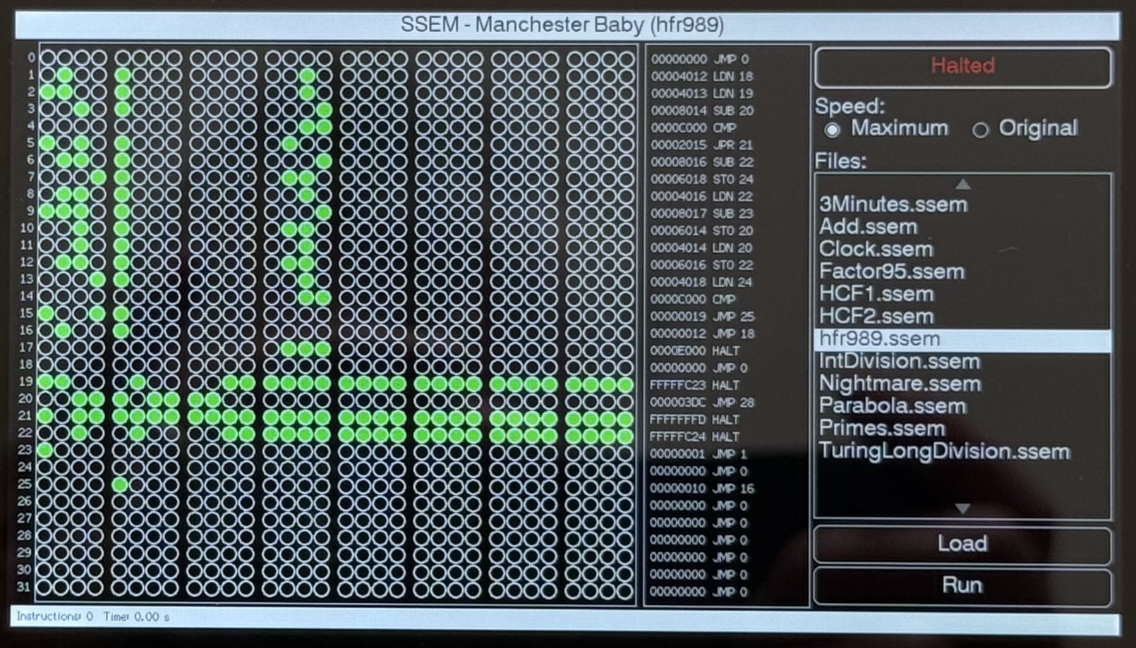
A few visual elements were overlapping, but a quick guiding prompt fixed the problem.
Case Study 3 – Explaining the Messaging System
Code does not always explain the full system. One project being developed uses a messaging system that uses the heap to pass messages between system components and the outside world. Copilot was asked to review the code and did a good job, picking up a couple of potential issues which were easily fixed.
There was, however, one false positive that turned up in a couple of places. Copilot picked up on the heap allocation of messages but reported that the memory was never released. It was necessary to explain that the messages were heap-allocated by one component but the memory was released by a different component.
Case Study 4 – Circles Of My Mind
A recent task required rebasing some firmware from an old version circa August 2023 to the latest shiny code base. The task started by merging one release at a time (12.3 -> 12.4; 12.4 -> 12.5 etc) until confidence in the process reached the level where jumping several versions at once was deemed possible. So let’s jump all the way to the latest version, 12.13.
Flash the firmware and the board faults in a boot loop. Time to roll back to the last known good and go back to one version at a time.
Finally located the fact that 12.12 to 12.13 was the culprit, 12.12 worked as expected, 12.13 caused the boot loop. A manual code review did not highlight any obvious issues and other users have the code running on many different boards. Maybe AI can help, we have two known release tags for the code so examining the differences along with information about the development board may lead to an answer.
A few hours and over 40 million tokens later, no result. What was observed on a couple of occasions was the AI making comments along the lines of “Wait, I’m going in circles here” – it happens to the best of us.
Time to stop the AI and apply some RI (Real Intelligence) to this problem.
Conclusion
There is no doubt that AI is here to stay. It is capable of producing code in large volumes and is a valuable development tool. It can give insights into existing code and, when carefully guided, can analyse complex problems faster than an experienced developer.
Having praised the virtues of AI, we should also be cautious. It is a junior developer and, as such, makes mistakes as we all did when we were junior developers. It is also a junior developer with an appalling memory, teach it something today and it will have forgotten it tomorrow (tell it to make notes in markdown files and get it to read them back the next day).
AI is really just a tool, one that is very different to the tools we have used in the past. Speaking as an experienced developer, used correctly it can improve productivity and code quality. I know I am seeing an increase in the number and type of tasks I am now completing.
We also need to be aware that humans are responsible for the quality of the code produced and as such we must take responsibility. We cannot blame the AI if the code is poor or it fails.