Embedded Developer

A while ago I put together an emulator for the Small Scale Experimental Machine (SSEM), also known as the Manchester Baby. This was a basic console application allowing a program written for the Manchester Baby to be run in a console application on a modern computer. As things turned out, I now spend most of my time working in either C or C++. This has left me with a piece of code that is difficult to maintain as I have to relearn Python every time I want to make any improvements.

Time to rewrite the application in C++.

SSEM Simulator

The simulator provides a number of features:

• Assembler/compiler to take source files and generate the binary to be execution
• Console interface to control the execution of the application
• Simulated display of the registers and memory

More information about the Python version of the simulator can be found in this blog and on the Small Scale Experimental Machine web site with full source code available on GitHub.

Porting the Simulator

The aim of the initial port is to provide the same functionality of the original application with any changes necessary to provide additional robustness as we are undoubtedly going to be seeing pointers in the C++ port.

Where possible, the structure of the original Python code has been maintained to keep a 1:1 mapping with the original code and test suite. This will provide an easy way to validate the unit tests in the port against the original Python code. The original Python code was validated against David Sharps Java Simulator.

The long term aim of this port is to provide a way of running the application on a Raspberry Pi Pico connected to hardware which will emulate the original SSEM. The application on the Raspberry Pi Pico will target the NuttX RTOS. As we will see later, compiling and running on NuttX will present some interesting issues.

Initial Port

The first stage of the port is to reproduce the core functionality of the SSEM showing the application output in a console interface targeting C++ 17. The only real complication here is ensure the user interface and platform specific code are abstracted to keep as much functionality in common with a desktop and NuttX implementation as possible.

The original Python code and the C++ port can be found in the Manchester Baby GitHub repository. A quick check of the source code shows that the 1:1 mapping has been kept where possible. The only real significant difference between the two code bases is the separation of the unit tests from the class implementation. The Python code keeps the unit test code in the class definitions themselves, the C++ code implements the unit tests in their own files.

Memory Checks

The switch from Python to C++ brings a new danger, memory access issues and memory leaks.

One memory issue that we can address relatively easily is memory leaks. If we can abstract the core functionality into a self contained group of files then we can use valgrind to check for memory leaks. A small glitch with using valgrind is that the application is not available for Mac from the key repositories. There is an informal project on GitHub.

The issue of valgrind not running on the mach was resolved by putting together a Dockerfile containing common development tools. The memory check could then be run on the desktop using Docker.

Running the Emulator

The emulator can be run on both a desktop computer as well as a board running NuttX.

Run from the Desktop

Running the application on the desktop is the simplest way to test the emulator:

• Open a command console and change to the Desktop directory in the repository
• Build the emulator with the command make
• Run the emulator with the command ./ssem_main

Run on NuttX

Running on NuttX is a little more complex as we need to build the application and the operating system and then deploy the binary to a board. The processes of adding the SSEM application to a Raspberry Pi PicoW board has already been documented in the article Adding a User Application to NuttX. The first step is to follow the steps in the article to add the SSEM basic applicatiom.

The next stage is to copy the contents of the NuttX directory over the application directory created in the above article. The code should then be rebuilt with the command make clean && make -j. The application can now be deployed to the board.

Now we have the OS and the application deployed to the Raspberry Pi (or your board of choice) we can connect a serial adapter to the board and press the enter key twice. This will bring up the NuttX shell. Typing help should show the ssem application deployed to the board. Simply execute this by entering the command ssem.

Application Output

In both cases the emulator should run the hfr989.ssem application (the source for this can be found in the SSEMApps folder in the repository). Both the desktop and the NuttX versions of the emulator will run the SSEM application and will show the start and end state of the SSEM on the console / serial port. The first output will show the SSEM application loaded into the store lines:

NuttShell (NSH) NuttX-10.4.0
nsh> ssem
                   00000000001111111111222222222233
                   01234567890123456789012345678901
   0: 0x00000000 - 00000000000000000000000000000000 JMP 0            ; 0
   1: 0x48020000 - 01001000000000100000000000000000 LDN 18           ; 16402
   2: 0xc8020000 - 11001000000000100000000000000000 LDN 19           ; 16403
   3: 0x28010000 - 00101000000000010000000000000000 SUB 20           ; 32788
   4: 0x00030000 - 00000000000000110000000000000000 CMP              ; 49152
   5: 0xa8040000 - 10101000000001000000000000000000 JPR 21           ; 8213
   6: 0x68010000 - 01101000000000010000000000000000 SUB 22           ; 32790
   7: 0x18060000 - 00011000000001100000000000000000 STO 24           ; 24600
   8: 0x68020000 - 01101000000000100000000000000000 LDN 22           ; 16406
   9: 0xe8010000 - 11101000000000010000000000000000 SUB 23           ; 32791
  10: 0x28060000 - 00101000000001100000000000000000 STO 20           ; 24596
  11: 0x28020000 - 00101000000000100000000000000000 LDN 20           ; 16404
  12: 0x68060000 - 01101000000001100000000000000000 STO 22           ; 24598
  13: 0x18020000 - 00011000000000100000000000000000 LDN 24           ; 16408
  14: 0x00030000 - 00000000000000110000000000000000 CMP              ; 49152
  15: 0x98000000 - 10011000000000000000000000000000 JMP 25           ; 25
  16: 0x48000000 - 01001000000000000000000000000000 JMP 18           ; 18
  17: 0x00070000 - 00000000000001110000000000000000 HALT             ; 57344
  18: 0x00000000 - 00000000000000000000000000000000 JMP 0            ; 0
  19: 0xc43fffff - 11000100001111111111111111111111 HALT             ; -989
  20: 0x3bc00000 - 00111011110000000000000000000000 JMP 28           ; 988
  21: 0xbfffffff - 10111111111111111111111111111111 HALT             ; -3
  22: 0x243fffff - 00100100001111111111111111111111 HALT             ; -988
  23: 0x80000000 - 10000000000000000000000000000000 JMP 1            ; 1
  24: 0x00000000 - 00000000000000000000000000000000 JMP 0            ; 0
  25: 0x08000000 - 00001000000000000000000000000000 JMP 16           ; 16
  26: 0x00000000 - 00000000000000000000000000000000 JMP 0            ; 0
  27: 0x00000000 - 00000000000000000000000000000000 JMP 0            ; 0
  28: 0x00000000 - 00000000000000000000000000000000 JMP 0            ; 0
  29: 0x00000000 - 00000000000000000000000000000000 JMP 0            ; 0
  30: 0x00000000 - 00000000000000000000000000000000 JMP 0            ; 0
  31: 0x00000000 - 00000000000000000000000000000000 JMP 0            ; 0

Reading from left to right, the above output shows the following:

• Store line number (i.e. the memory address) 0:, 1: etc.
• The hexadecimal representation of the store line contents.
• Binary representation of the store line contents
• Disassembled representation of the store line contents JMP 0 etc.
• Decimal representation of the store line contents

It must be remembered when reading the above that the least significant bit is at the left of the word and the most significant bit is to the right. This is honoured with the hexadecimal and binary components of the above output. The decimal value to the right should be read in the usual way for a base 10 number.

After a short time the contents of the store lines at the end of the run will be displayed:

Program execution complete.
                   00000000001111111111222222222233
                   01234567890123456789012345678901
   0: 0x00000000 - 00000000000000000000000000000000 JMP 0            ; 0
   1: 0x48020000 - 01001000000000100000000000000000 LDN 18           ; 16402
   2: 0xc8020000 - 11001000000000100000000000000000 LDN 19           ; 16403
   3: 0x28010000 - 00101000000000010000000000000000 SUB 20           ; 32788
   4: 0x00030000 - 00000000000000110000000000000000 CMP              ; 49152
   5: 0xa8040000 - 10101000000001000000000000000000 JPR 21           ; 8213
   6: 0x68010000 - 01101000000000010000000000000000 SUB 22           ; 32790
   7: 0x18060000 - 00011000000001100000000000000000 STO 24           ; 24600
   8: 0x68020000 - 01101000000000100000000000000000 LDN 22           ; 16406
   9: 0xe8010000 - 11101000000000010000000000000000 SUB 23           ; 32791
  10: 0x28060000 - 00101000000001100000000000000000 STO 20           ; 24596
  11: 0x28020000 - 00101000000000100000000000000000 LDN 20           ; 16404
  12: 0x68060000 - 01101000000001100000000000000000 STO 22           ; 24598
  13: 0x18020000 - 00011000000000100000000000000000 LDN 24           ; 16408
  14: 0x00030000 - 00000000000000110000000000000000 CMP              ; 49152
  15: 0x98000000 - 10011000000000000000000000000000 JMP 25           ; 25
  16: 0x48000000 - 01001000000000000000000000000000 JMP 18           ; 18
  17: 0x00070000 - 00000000000001110000000000000000 HALT             ; 57344
  18: 0x00000000 - 00000000000000000000000000000000 JMP 0            ; 0
  19: 0xc43fffff - 11000100001111111111111111111111 HALT             ; -989
  20: 0x54000000 - 01010100000000000000000000000000 JMP 10           ; 42
  21: 0xbfffffff - 10111111111111111111111111111111 HALT             ; -3
  22: 0x6bffffff - 01101011111111111111111111111111 HALT             ; -42
  23: 0x80000000 - 10000000000000000000000000000000 JMP 1            ; 1
  24: 0x00000000 - 00000000000000000000000000000000 JMP 0            ; 0
  25: 0x08000000 - 00001000000000000000000000000000 JMP 16           ; 16
  26: 0x00000000 - 00000000000000000000000000000000 JMP 0            ; 0
  27: 0x00000000 - 00000000000000000000000000000000 JMP 0            ; 0
  28: 0x00000000 - 00000000000000000000000000000000 JMP 0            ; 0
  29: 0x00000000 - 00000000000000000000000000000000 JMP 0            ; 0
  30: 0x00000000 - 00000000000000000000000000000000 JMP 0            ; 0
  31: 0x00000000 - 00000000000000000000000000000000 JMP 0            ; 0
Executed 21387 instructions in 30000000 nanoseconds

The original SSEM ran at about 700 instructions per second, modern PCs and even RP2040 processors are running the application much faster.

Conclusion

Even small boards (such as the Raspberry Pi Pico) running relatively low power processors can now emulate the Manchester Baby running application intended for the SSEM many times faster that the original hardware. The hfr989.ssem application would have run in about 30 seconds in 1948, today we can run this in an emulator in less that 30ms.

One feature that I want to add to my current project is to add a small file system with files that have been built into the system at compile time. These files would then be available to the application at run time. Let’s look at how we can do can do this with NuttX.

This tutorial assumes that you have NuttX cloned and ready to build, if not then you can find out how to do this in the first article in this series.

Adding SmartFS to the Build

NuttX has a built in configuration for the PicoW with SmartFS already configured. The first thing we need to do is to start with a clean system and then configure the build to include NSH and the flash file system. Start by changing to the NuttX source directory and then executing the following commands:

make distclean
./tools/configure.sh -l raspberrypi-pico-w:nsh-flash

Now we have the system configured we can build the OS and applications by executing the following command:

make -j

This should take a minute or so on a modern machine. Now we can deploy the system to the PicoW either by using openocd or by dragging the uf2 file onto the PicoW drive. Now connect to the PicoW using a serial application and type help to show the menu of commands. You should see something like the following:

SmartFS Builtin Apps

We can check to see if the SmartFS is available checking the contents of the /dev directory with the command ls /dev. This should result in something like the following if SmartFS has been enabled correctly:

Device Directory Listing

We can mount the file system using the command mount -t smartfs /dev/smart0 /data and then check the contents of the /data directory and we should find one file in the directory, test. Checking the contents of the file with the command cat /data/test should find that it contains a single ine of text which should be Hello, world!.

So far, so good, we have built the system and proven that it contains the default file and correct contents.

Adding a New File to the System Image

The next piece of the puzzle is to work out how to add new files to the file system. This took a few hours to figure out, but here goes…

The first attempt lead me searching for RP2040_FLASH_FILE_SYSTEM in the source tree (ripgrep is a great tool for doing this). This lead to a number of possible files. Maybe we can narrow the search down a little.

Second attempt, let’s have a look for Hello, world!. This resulted in a smaller number of files leading to the file arch/arm/src/rp2040/rp2040_flash_initialize.S. This file is well documented and shows how to set up the SmartFS file system and at the end of the file it shows how to create an entry for the file we see when we list the mounted directory. Scrolling down to the end of the fie we find the following:

    sector      3, dir
    file_entry  0777, 4, 0, "test"

    sector      4, file, used=14
    .ascii      "Hello, world!\n"

    .balign     4096, 0xff
    .global     rp2040_smart_flash_end
rp2040_smart_flash_end:

This looks remarkably familiar. So what happens if we change the above to look like this:

    sector      3, dir
    file_entry  0777, 4, 0, "test"
    file_entry  0777, 5, 0, "test2"

    sector      4, file, used=14
    .ascii      "Hello, world!\n"

    sector      5, file, used=14
    .ascii      "Testing 1 2 3\n"

    .balign     4096, 0xff
    .global     rp2040_smart_flash_end
rp2040_smart_flash_end:

Building the system, deploying the code and executing the following commands:

mount -t smartfs /dev/smart0 /data
cd /data
ls

results in the following:

New file added to SmartFS

If we execute the command cat test2 we are rewarded with the output Testing 1 2 3.

Further testing shows that the file system survives through a reset. We can do the following:

• echo “My test” > test3
• rm test
• reboot

These commands should remove the file test, create a new file test3 and then reboot the system. Checking the file system contents shows that the system persists the changes through a reset.

Conclusion

This experiment was a partial success. A simple file system has been made available to an application and the file system survives a reset. One issue remains, adding new files is a little complex. It also requires changes to the NuttX source tree outside of the applications folder. This could result in changes being lost when a new version of NuttX is released.

There could be a solution, ROMFS, stay tuned for the next episode.

In the previous post, we managed to get GDB working with NuttX running on the Raspberry Pi PicoW. In this post we will look at using VSCode to debug NuttX.

For a large part of this post it was case of following Shawn Hymels guide Raspberry Pi Pico and RP2040 – C/C++ Part 2 Debugging with VS Code. This is an excellent guide and I recommend using it as a companion to this post.

We will start with the assumption that you have followed the previous post in this series and have a working NuttX build for the Raspberry Pi PicoW. We will also assume that you have a working VSCode installation with the Cortex-Debug extension installed.

Configuration Files

We will need to create (or modify) three configuration files to allow VSCode to debug NuttX.

• launch.json
• tasks.json
• settings.json

In the first article of this series we created the directory NuttX-PicoW to hold the apps and nuttx folders holding out NuttX code. This directory is the project directory or in VS Code parlance, the workspaceFolder. The workspaceFolder should also contain the Raspberry Pi PicoW SDK and the Raspberry Pi specific version of openocd.

We now add a .vscode directory to the workspaceFolder. This directory will hold the three configuration files listed above.

Start by opening VS Code and opening the workspaceFolder. This should show the four folders already in the workspaceFolder. Now create a .vscode directory in the workspaceFolder if it does not already exist.

setting.json

Only one entry is required in the settings.json file and this is the location of the openocd executable. If you have followed these posts so far this will be in the openocd/src folder. Create a setting.json file in the .vscode folder and add the following to the file.

{
    "cortex-debug.openocdPath": "${workspaceFolder}/openocd/src/openocd"
}

Note that the name of the executable may vary depending upon your operating system this post is being written from a MacOS perspective.

tasks.json

The tasks.json file holds the entry that will be used to build NuttX prior to deployment. In Shawns document the projects being worked on use the cmake system. We need to modify this to build NuttX using make. We want VS Code to use the command make -C ${workspaceFolder}/nuttx -j to build NuttX. The build task below will create a task Build NuttX to do just this:

{
    "version": "2.0.0",
    "tasks": [
        {
          "label": "Build NuttX",
          "type": "cppbuild",
          "command": "make",
          "args": [
            "-C",
            "${workspaceFolder}/nuttx",
            "-j"
          ]
        }
      ]  
}

launch.json

Of the three files we are creating, the launch.json file is the most complex. Much of the file remains the same as that presented by Shawn but there are some differences. The file used here looks like this:

{
    "version": "0.2.0",
    "configurations": [
        {
            "name": "Pico Debug",
            "cwd": "${workspaceRoot}",
            "executable": "${workspaceFolder}/nuttx/nuttx.elf",
            "request": "launch",
            "type": "cortex-debug",
            "servertype": "openocd",
            "gdbPath" : "arm-none-eabi-gdb",
            "device": "RP2040",
            "configFiles": [
                "interface/cmsis-dap.cfg",
                "target/rp2040.cfg"
            ],
            "svdFile": "${workspaceFolder}/pico-sdk/src/rp2040/hardware_regs/rp2040.svd",
            "runToEntryPoint": "__start",
            "searchDir": ["${workspaceFolder}/openocd/tcl"],
            "openOCDLaunchCommands": ["adapter speed 5000"],
            "preLaunchTask": "Build NuttX"
        }
    ]
}

The following items are the ones that need to be changed:

“executable”: “${workspaceFolder}/nuttx/nuttx.elf”

This is the path to the executable that will be created by the build system. In this cse it is the NuttX ELF file. This may need to be changed to “executable”: “${workspaceFolder}/nuttx/nuttx” depending upon the output of the build system, this may simply be nuttx.

“configFiles”

The recent versions of the picoprobe software use a different interface to talk to the picoprobe. For versions 1.01 and above of the picoprobe software this interface changed from picoprobe.cfg to cmsis-dap.cfg.

“svdFile”: “${workspaceFolder}/pico-sdk/src/rp2040/hardware_regs/rp2040.svd”

We have a version of the Pico SDK specifically for our build requirements and so for this reason the location of the file is changed to reference the workspaceFolder rather than the global PICO_SDK_PATH environment variable.

“runToEntryPoint”: “__start”

This entry replaces the “runToMain”: true entry. Unlike convention C/C++ applications, NuttX does not have a main method. Having the runToMain entry generates an error stating that main cannot be found and stops at the first executable statement in our code, namely in __start. Replacing runToMain with runToEntryPoint achieves the same thing but does not generate the error.

Doing this also removes the need to have the postRestartCommands specified.

“searchDir”: [“${workspaceFolder}/openocd/tcl”]

This entry is used by openocd to look for the interface and target configuration files specified in the configFiles entry.

“openOCDLaunchCommands”: [“adapter speed 5000”]

These commands are executed by openocd when it starts. The change to the adapter speed is required and is documented in Getting Started with Raspberry Pi Pico documentation from the Raspberry Pi Foundation.

“preLaunchTask”: “Build NuttX”

The final entry tells Cortex-Debug how to build NuttX. It references the task we previously defined in the tasks.json file.

Testing

Testing this should simply be a case of saving all of the files above and pressing F5 in VS Code. If the changes have been successful then VS Code will first try to build NuttX in a Terminal window and it will then deploy NuttX to the Pico board and start the debugger. VS Code should look something like this (click on image for full view):

Debugging PicoW with VSCode

The inclusion of the SVD file allows us to examine the PicoW peripheral registers as well as the core registers:

PicoW Peripheral Registers in VSCode	Pico Cortex Registers in VSCode

Conclusion

GDB is a great debugger but it is often more convenient to use an IDE to debug your code. VS Code with the Cortex-Debug extension allow visual debugging of NuttX with a few nice additional features thrown in:

• Easily viewed call stacks for both cores.
• The SVD file allows the peripheral registers to be viewed through VS Code

We should also note that the use of VS Code resolved the issues noted at the end of the previous post as Cortex-Debug is able to deploy a binary using the picoprobe without resorting to the UF2 method of deployment. This results in a seamless build, deploy and debug process.

We have two debug options and it is now down to personal preferences as to which one to use.

One of the current projects on the go is a level shifter for the Teensy 3.6 using the TXS0108E chip. The aim is to allow the use of as many of the Teensy’s GPIO pins as possible to allow the development of another project that is working on 5V logic levels.

This project reminded me that when putting together a microcontroller project that the system is made up of both hardware and software. Sometimes a design decision made in one element can have an adverse effect on the other.

Design Decisions

From the start it was decided that the GPIO pins would have a one to one mapping from the microcontroller to the external bus. So pin 1 on the microcontroller would map to pin 1 on the external connectors.

This would make coding easy when using the Arduino API. So connecting to the external bus and outputting a digital high signal on pin 1 would become:

pinMode(1, OUTPUT);
digitalWrite(1, HIGH);

Impact

Putting the circuit together in KiCAD resulted in the following design:

PCB Layout

TXS0108E Schematic

As you can see, the Teensy GPIOS (TIO-1…) mapped directly to the external bus (GPIO-1…)

When translated into the rats nest there were three occurrences of the following:

PCB Layout

Routing this was going to be a nightmare.

Changing the Design

At this point the penny dropped that a small change in the software would make the routing a whole lot easier.

Instead of using the pin numbers directly, a #define could be used for the external bus pin numbers. The above snippet would become:

#define BUS_IO1    30
.
.
.
pinMode(BUS_IO1, OUTPUT);
digitalWrite(BUS_IO1, HIGH);

This small change to the design created a one off task to create a header file for the board but it made the routing a lot easier.

Conclusion

Sometimes a small change may create a new task (creating the header file) but may possibly save more time elsewhere in the project.

Moral of the story, Design the system as a whole, not the individual components.

The Manchester Small Scale Experimental Machine (SSEM) or Manchester Baby as it became known, was the first computer capable of executing a stored program. The Baby was meant as a proving ground for the early computer technology having only 32 words of memory and a small instruction set.

A replica of the original Manchester Baby is currently on show in the Museum of Science and Industry in Castlefield, Manchester.

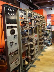
Manchester Baby at Museum of Science and Industry August 2012.

As you can see, it is a large machine weighing in at over 1 ton (that’s imperial, not metric, hence the spelling).

Manchester Baby Architecture

A full breakdown on the Manchester Baby’s architecture can be found in the Wikipedia article above as well as several PDFs, all of which can be found online. The following is meant as a brief overview to present some background to the Python code that will be discussed later.

Storage Lines

Baby used 32-bit words with numbers represented in twos complement form. The words were stored in store lines with the least significant bit (LSB) first (to the left of the word). This is the reverse of most modern computer architectures where the LSB is held in the right most position.

The storage lines are equivalent to memory in modern computers. Each storage line contains a 32-bit value and the value could represent an instruction or data. When used as an instruction, the storage line is interpreted as follows:

As already noted, when the storage line is interpreted as data then the storage line contains a 32-bit number stored in twos complement form with the LSB to the left and the most significant bit (MSB) to the right.

This mixing of data and program in the same memory is known as von Neumann architecture named after John von Neumann. For those who are interested, the memory architecture where program and data are stored in separate storage areas is known as a Harvard architecture.

SSEM Instruction Set

Baby used three bits for the instruction opcode, bits 13, 14 and 15 in each 32 bit word. This gave a maximum of 8 possible instructions. In fact, only seven were implemented.

When reading the above table it is important to remember that the LSB is to the left.

Registers

Baby had three storage areas within the CPU:

1. Current Instruction (CI)
2. Present Instruction (PI)
3. Accumulator

The current instruction is the modern day equivalent of the program counter. This contains the address of the instruction currently executing. CI is incremented before the instruction is fetched from memory. At startup, CI is loaded with the value 0. This means that the first instruction fetched from memory for execution is the instruction in storage line 1.

The present instruction (PI) is the actual instruction that is currently being executed.

As with modern architecture, the accumulator is used as a working store containing the results of any calculations.

Python Emulator

A small Python application has been developed in order to verify my understanding of the architecture of the Manchester Baby. The application is a console application with the following brief:

1. Read a program from a file and setup the store lines
2. Display the store lines and registers before the program starts
3. Execute the program displaying the instructions as they are executed
4. Display the store lines and registers at the end of the program run

The application was broken down into four distinct parts:

1. Register.py – implement a class containing a value in a register or storage line
2. StoreLines.py – Number of store lines containing the application and data
3. CPU.py – Implement the logic of the CPU
4. ManchesterBaby.py – Main program logic, reading a program from file and executing the program

The source code for the above along with several samples and test programs can be fount on Github.

Register.py

A register is defined as a 32-bit value. The Register class stores the value and has some logic for checking that the value passed does not exceed the value permitted for a 32-bit value. Note that no other checks or interpretation of the value is made.

StoreLines.py

StoreLines holds a number of Registers, the default when created is 32 registers as this maps on to the number of store lines in the original Manchester Baby. It is possible to have a larger number of store lines.

CPU.py

The CPU class executes the application held in the store lines. It is also responsible for displaying the state of the CPU and the instructions being executed.

ManchesterBaby.py

The main program file contains an assembler (a very primitive one with little error checking) for the Baby’s instruction set. It allows a file to be read and the store lines setup and finally instructs the CPU to execute the program.

SSEM Assembler Files

The assembler provided in the ManchesterBaby.py file is primitive and provides little error checking. It is still useful for loading applications into the store lines ready for execution. The file format is best explained by examining a sample file:

--
--  Test the Load and subtract functions.
--
--  At the end of the program execution the accumulator should hold the value 15.
--
00: NUM 0
01: LDN 20      -- Load accumulator with the contents of line 20 (-A)
02: SUB 21      -- Subtract the contents of line 21 from the accumulator (-A - B)
03: STO 22      -- Store the result in line 22
04: LDN 22      -- Load accumulator (negated) with line 22 (-1 * (-A - B))
05: STOP        -- End of the program.
20: NUM 10      -- A
21: NUM 5       -- B
22: NUM 0       -- Result

Two minus signs indicate an inline comment. Everything following is ignored.

An instruction line has the following form:

Store line number: Instruction Operand

The store line number is the location in the Store that will be used hold the instruction or data.

Instruction is the mnemonic for the instruction. The some of the instructions have synonyms:

As well as instructions a number may also be given using the NUM mnemonic.

All of the mnemonics requiring a store number (all except STOP and CMP) read the Operand field as the store line number. The NUM mnemonic stores the Operand in the store line as is.

Testing

Testing the application was going to be tricky without a reference. Part of the reason for developing the Python implementation was to check my understanding of the operation of the SSEM. Luckily, David Sharp has developed an emulator written in Java. I can use this to check the results of the Python code.

The original test program run on the Manchester Baby was a calculation of factors. This was used as it would stress the machine. This same application can be found in several online samples and will be used as the test application. The program is as follows:

--
--  Tom Kilburns Highest Common Factor for 989
--
01:   LDN 18
02:   LDN 19
03:   SUB 20
04:   CMP
05:   JRP 21
06:   SUB 22
07:   STO 24
08:   LDN 22
09:   SUB 23
10:   STO 20
11:   LDN 20
12:   STO 22
13:   LDN 24
14:   CMP
15:   JMP 25
16:   JMP 18
17:   STOP
18:   NUM 0
19:   NUM -989
20:   NUM 988
21:   NUM -3
22:   NUM -988
23:   NUM 1
24:   NUM 0
25:   NUM 16

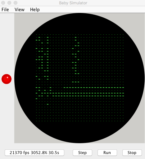
Running on the Java Emulator

Executing the above code in David Sharps emulator gives the following output on the storage tube:

Result of the HCF application shown on the storage lines of the Java emulator.

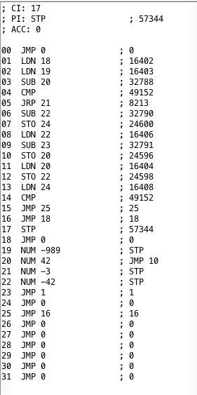
and disassembler view:

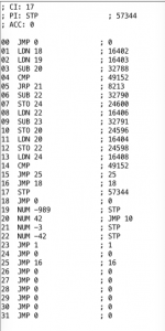
Result of the program execution disassembled in the Java emulator.

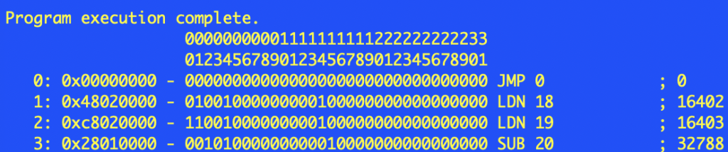
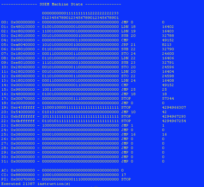
And running on the Python version of the emulator results in the following output in the console:

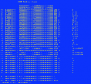
Final output from the Python emulator.

Examination of the output shows that the applications have resulted in the same output. Note that the slight variation in the final output of the Python code is due to the way in which numbers are extracted from the registers. Examination of the bit patterns in the store lines shows that the Java and Python emulators have resulted in the same values.

Conclusion

The Baby presented an ideal way to start to examine computer architecture due to its prmitive nature. The small storage space and simple instruction set allowed emulation in only a few lines of code.

The weather station project has been struggling for part of September with a random exception in my code. The source of the exception was finally identified although the exact cause is still a mystery. As a temporary measure, the component and the associated source code were removed from the project, this allowed the project to continue.

Source of the Exception

In the previous post, Define a Minimum Viable Product and Ship it, I discussed a replacement for the clock module. This module was changed from the DS3234 to the DS3231 freeing up four additional pins (the DS3231 is an I2C peripheral and the DS3234 uses SPI). This change seems to have introduced some instability into the system.

Several days debugging followed after which I was still unable to isolate the problem. The interim solution is to remove the module and use the Ticker class to trigger an interrupt. Not ideal but this will allow the rest of the software to be soak tested.

The additional Ticker object fires once per minute to trigger the reading of the sensors. In addition, the interrupt will check the current time and if the hour and minute are both zero then the application will reset the pluviometer counter.

Soak Testing

As mentioned above, one Ticker object is generating an interrupt once per minute. The frequency of the interrupt is higher than will be used in the final project. One minute is more than enough time to perform the sensor readings and log this to the internet but also frequent enough to simulate a prolonged period in the field.

The prototype board was also located close to the final home for the sensors. This hit a problem as the range of the WiFi network was not sufficient for the ESP8266. This problem has prevented the prototype to be tested in the field at the moment.

Conclusion

The prototype board is currently sited on a window ledge in the house. taking temperature, humidity and luminosity readings once per minute. This data is logged to the Sparkfun Phant Data Service. The system has been running continuously for the last 7 days (approximately 10,000 readings).

The software seems stable at the moment, the next problem, extend the range of the WiFi network.

The last few weeks have seen me fighting a communication problem between the Oak and the STM8S. As a result the development has slowed down a little to the point that the project was becoming frustrating. It was about two weeks ago that I was listening to a podcast and the presenter made a very pertinent comment. Some software start-ups fail because they fail to define the minimum viable product. This gives them nothing to aim for and most importantly no firm idea of what they have to deliver.

This felt very relevant as the weather station was stalling. With this in mind I decided to break the project up into a number of revisions.

Revision One – Basic Sensing

Although this revision is titled Basic Sensing, we will aim to get as many of the sensors working with the Oak, and only the Oak, as possible.

The Oak has an ESP8266 (ESP12) at it heart and this leaves a restricted number of IO pins available to communicate with the outside world. With this in mind it should still be possible to work with the following sensors:

1. Wind speed and direction
2. Pluviometer
3. BME280 (air temperature, humidity and temperature)
4. DS18B20 (ground temperature
5. TSL2561 (luminosity)

An additional pin is also required to allow the Real Time Clock (RTC) module to generate and interrupt to let the Oak know it is time to take a reading.

One of the aims of the final system is to be able to run using solar power and batteries, however, for the initial version of the system this is not necessary. The main controller board can be placed inside to run on mains power with the rain and wind sensors outside. Some of the sensors would be inside so this would not give a good view of the weather but will allow testing of the software.

Clock Module Change

I came across a variant of the DS3234 RTC on one of my usual suppliers web page. The DS3231 module is similar to the DS3234 with four differences:

1. Price – I can buy four of the DS3231 modules for the same price as one DS3234
2. Interface – the DS3231 uses I2C rather than SPI
3. No on chip memory for the DS3231
4. Additional EEPROM on board

All of the main features that make the DS3234 desirable are also present in the DS3231. The major piece of work is the necessity to overhaul the DS3234 library created previously.

Schematic

The main changes to the hardware design involve moving the connections to the various sensors from the STM8S to the Oak. This has been made possible by the change in the clock module from the DS3234 (SPI) to the DS3231 (I2C). This freed up the four pins that had been dedicated to the SPI interface.

The updated schematic is as follows:

Weather Station Rev1 Schematic

Translating this to hardware on a protoboard:

Weather Station Rev1 Protoboard

There are a couple of items on the hardware implementation that are not on the schematic:

• Additional connectors / jumpers
• Connector for OpenLog board

These items may or may not make it onto the final board and have been added to aid debugging.

Software

The software for this project has been placed on Github and is broadly speaking the same as previous versions in terms of design. The following are the most significant changes:

1. STM8S code has been left in the project for the moment but this is not used in this initial working version.
2. Interrupts for the pluviometer and the wind speed are now in the Oak code
3. Logging to Phant has been implemented (public stream can be found
4. DS3234 code has been abstracted and used to make a DS323x generic timer class and a DS3231 specific class

One of the long term aims of the weather station is to take the system off grid. This will mean using an alternative energy source, something other than mains electricity. This usually means using solar energy to charge batteries in order to keep the system running.

Another scenario that will need to be considered is the case where the weather station is collecting data but is unable to connect to the internet. In this case it is desirable for the weather station to continue to collect data, record the date and time the observation was made and also store the readings. The system can then upload the data when the network connection is once available once more.

This article presents a possible solution to one problem and a possible solution to another:

1. Reducing power by putting the system to sleep
2. Recording the date / time when the system is not connected to the Internet

The solution being considered is a Real Time Clock (RTC) module based upon the DS3234 chip.

DS3234 RTC

The DS3234 is a real time clock module with a built in temperature controlled oscillator. It is a relatively self-contained module requiring few external components. The chip is programmed over the built in SPI interface.

A summary of the important features being considered are:

1. Built in alarm(s)
2. Battery back up
3. Built in oscillator
4. Interrupt on alarm

One additional feature that may be useful is the provision of 256 bytes of battery backed up RAM.

The interrupt generated by the alarms can be used to trigger the Oak to take action. In this way it may be possible for the Oak to sleep for a period of time waiting for a signal from the RTC. The RTC will run in much lower power mode than the Oak.

One disadvantage of this module, at the time of writing, was the lack of code that would either provide the functioality required or work reliably on the Oak.

Time to break out the C++ compiler.

Controlling the DS3234

Before we look at the software, it is worth spending a little time to review how the DS3234 is controlled. The RTC chip uses write operations to a series of registers in order to control the functionality of the chip. The register map is as follows:

Applications can write to the registers by setting bit 7 (i.e. add 0x80) in the address.

The register address is automatically incremented after a read or write operation. So to write the current time into the hours, minutes and seconds registers an application would simply write four bytes to the SPI bus; namely address 0x80 (write address for the seconds register) followed by the seconds, minutes and hour values.

The bit fields for the above registers are well defined in the DS3234 datasheet and are not covered in too much detail here and you are encouraged to download the datasheet for reference.

DS3234 Software – Private Interface

The full source code for this module can be downloaded from at the end of this article, the discussion about the software and it’s functionality will concentrate on the class definition in the header file. Those interested in the detail can jump into the source code at the end of the article.

So let’s have a look at the full header file:

#ifndef _DS3234_h
#define _DS3234_h

#include <BitBang\BitBang.h>

#if defined(ARDUINO) && ARDUINO >= 100
	#include "arduino.h"
#else
	#include "WProgram.h"
#endif

#define MAX_BUFFER_SIZE     256

//
//  Time structure.
//
struct ts
{
    uint8_t seconds;    // Number of seconds, 0-59
    uint8_t minutes;    // Number of minutes, 0-59
    uint8_t hour;       // Number of hours, 0-23
    uint8_t day;        // Day of the month, 1-31
    uint8_t month;      // Month of the year, 1-12
    uint16_t year;      // Year >= 1900
    uint8_t wday;       // Day of the week, 1-7
};

//
//  Define the methods required to communicate with the DS3234 Real Tiem Clock.
//
class DS3234RealTimeClock
{
    public:
        //
        //  Enums.
        //
        enum Alarm { Alarm1, Alarm2, Both, Unknown };
        enum AlarmType { OncePerSecond, WhenSecondsMatch, WhenMinutesSecondsMatch,  // Alarm 1 options.
                         WhenHoursMinutesSecondsMatch, WhenDateHoursMinutesSecondsMatch, WhenDayHoursMinutesSecondsMatch,
                         OncePerMinute, WhenMinutesMatch, WhenHoursMinutesMatch,    // Alarm 2 options.
                         WhenDateHoursMinutesMatch, WhenDayHoursMinutesMatch };
        enum ControlRegisterBits { A1IE = 0x01, A2IE = 0x02, INTCON = 0x04, RS1 = 0x08, RS2 = 0x10, Conv = 0x20, BBSQW = 0x40, NotEOSC = 0x80 };
        enum StatusRegisterBits { A1F = 0x02, A2F = 0x02, BSY = 0x04, EN32Khz = 0x08, Crate0 = 0x10, Crate1 = 0x20, BB32kHz = 0x40, OSF = 0x80 };
        enum RateSelect { OneHz = 0, OnekHz = 1, FourkHz = 2, EightkHz = 3 };
        enum Registers { ReadAlarm1 = 0x07, WriteAlarm1 = 0x87,
                         ReadAlarm2 = 0x0b, WriteAlarm2 = 0x8b,
                         ReadControl = 0x0e, WriteControl = 0x8e,
                         ReadControlStatus = 0x0f, WriteControlStatus = 0x8f,
                         ReadAgingOffset = 0x10, WriteAgingOffset = 0x90, 
                         ReadSRAMAddress = 0x18, WriteSRAMAddress = 0x98,
                         ReadSRAMData = 0x19, WriteSRAMData = 0x99 };
        enum DayOfWeek { Sunday = 1, Monday, Tuesday, Wednesday, Thursday, Friday, Saturday };
        //
        //  Construction and destruction.
        //
        DS3234RealTimeClock(const uint8_t);
        DS3234RealTimeClock(const uint8_t, const uint8_t, const uint8_t, const uint8_t);
        ~DS3234RealTimeClock();
        //
        //  Methods.
        //
        uint8_t GetAgingOffset();
        void SetAgingOffset(uint8_t);
        float GetTemperature();
        uint8_t GetControlStatusRegister();
        void SetControlStatusRegister(uint8_t);
        uint8_t GetControlRegister();
        void SetControlRegister(uint8_t);
        ts *GetDateTime();
        Alarm WhichAlarm();
        void SetDateTime(ts *);
        String DateTimeString(ts *);
        void SetAlarm(Alarm, ts *, AlarmType);
        void InterruptHandler();
        void ClearInterrupt(Alarm);
        void EnableDisableAlarm(Alarm, bool);
        void WriteToSRAM(uint8_t, uint8_t);
        uint8_t ReadFromSRAM(uint8_t);
        void ReadAllRegisters();
        void DumpRegisters(const uint8_t *);
        void ReadSRAM();
        void DumpSRAM();

    private:
        //
        //  Constants.
        //
        static const int REGISTER_SIZE = 0x14;
        static const int DATE_TIME_REGISTERS_SIZE = 0x07;
        static const int MEMORY_SIZE = 0xff;
        //
        //  Variables
        //
        int m_ChipSelect = -1;
        int m_MOSI = -1;
        int m_MISO = -1;
        int m_Clock = -1;
        uint8_t m_Registers[REGISTER_SIZE];
        uint8_t m_SRAM[MEMORY_SIZE];
        BitBang *m_Port;
        //
        //  Make the default constructor private so it cannot be called explicitly.
        //
        DS3234RealTimeClock();
        //
        //  Methods.
        //
        void Initialise(const uint8_t, const uint8_t, const uint8_t, const uint8_t);
        void SetRegisterValue(const Registers, uint8_t);
        uint8_t GetRegisterValue(const Registers);
        uint8_t ConvertUint8ToBCD(const uint8_t);
        void BurstTransfer(uint8_t *, uint8_t);
        void BurstTransfer(uint8_t *, uint8_t *, uint8_t);
        uint8_t ConvertBCDToUint8(const uint8_t);
};

#endif

Perversely, this discussion will start with the private data items and methods as these underpin the way in which the class provides the higher-level functionality.

Constants

The three constants define the size of the various register and RAM space within the chip.

REGISTER_SIZE

Defines the total number of bytes in the register bank excluding the reserved and SRAM registers.

DATE_TIME_REGISTERS_SIZE

Number of bytes holding the current date and time information.

MEMORY_SIZE

Number of bytes of SRAM.

Private Member Variables

The private member variables hold the state information for the class.

As noted in the datasheet for the DS3234, communication with the DS3234 is over the SPI bus. The first version of this class uses a software SPI class BitBang to provide this functionality.

m_Clock, m_MOSI, m_MISO, m_ChipSelect

The software SPI class allows the user to change the pins that provide the MOSI, MISO and Clock input/outputs. These four member variables record the pins used to provide the soft SPI bus.

m_Port

Instance of the class providing the SPI service.

m_Registers

Internal copy of the registers (up to the reserved registers).

m_SRAM

Internal copy of the SRAM.

Methods

The private methods provide the low level functionality supporting the public methods. These methods provide functions such as initialisation, communication and data conversion.

DS3234RealTimeClock()

The default constructor is made private to ensure that the developer cannot call this accidentally, forcing the use of the constructors that define the properties of the soft SPI bus.

void Initialise(const uint8_t chipSelect, const uint8_t mosi, const uint8_t miso, const uint8_t clock)

The four parameters inform the class which pins are used for the MOSI, MISO, Clock and Chip Select functions.

uint8_t ConvertBCDToUint8(const uint8_t value)

The values in the registers recording the date / time hold BCD values. This method provides a way to convert the DS3234 BCD values into a more natual (for the developer) uint8_t value.

uint8_t ConvertUint8ToBCD(const uint8_t value)

As noted above (see ConvertBCDToUint8), the DS3234 uses BCD to hold time vales. This methods provdes a method to convert uint8_t values to BCD before they are written to the registers.

uint8_t GetRegisterValue(const Registers reg)

Read a value from the specified register.

void SetRegisterValue(const Registers reg, const uint8_t value)

Set the specified register reg to value.

void BurstTransfer(uint8_t *dataToChip, uint8_t size) and void BurstTransfer(uint8_t *dataToChip, uint8_t *dataFromChip, uint8_t size)

As noted in the hardware discussion, the DS3234 will automatically increment the “address register” if multiple bytes of data are written to the SPI bus. These two methods take advantage of this functionality.

The first variant of the overloaded method, BurstTransfer(uint8_t *dataToChip, uint8_t size), transfers a number of bytes defined by size to the SPI bus. No data is read from the bus.

In both cases, the first byte of the dataToChip buffer is set to the address of the first register to be read/written.

DS3234 Software – Public Interface

The public interface is the useful part of this class as it provides the functionality that is usable by the application developer.

Enumerated Types

The first group of items in the public interface are a series of enumerated types. These allow a meaningful name to be given to the various registers, bits within the registers and method parameters.

Alarm

There are two alarms on the DS3234, Alarm1 and Alarm2. These have slightly different capabilities as defined in the next enum.

enum Alarm { Alarm1, Alarm2, Both, Unknown };

This enum is also used to represent the type of alarm that has been generated.

AlarmType

The AlarmType represents the type of alarm being set. These have been put into two groups, one for each of the alarms:

enum AlarmType { OncePerSecond, WhenSecondsMatch, WhenMinutesSecondsMatch,  // Alarm 1 options.
                 WhenHoursMinutesSecondsMatch, WhenDateHoursMinutesSecondsMatch, WhenDayHoursMinutesSecondsMatch,
                 OncePerMinute, WhenMinutesMatch, WhenHoursMinutesMatch,    // Alarm 2 options.
                 WhenDateHoursMinutesMatch, WhenDayHoursMinutesMatch };

The first two lines represent the type of alarms that can be set on Alarm1, the second two lines can be used with Alarm2.

ControlRegisterBits

The values in this enum are the flags in the control register:

enum ControlRegisterBits { A1IE = 0x01, A2IE = 0x02, INTCON = 0x04, RS1 = 0x08, RS2 = 0x10, Conv = 0x20, BBSQW = 0x40, NotEOSC = 0x80 };

Two or more options can be set by or-ing the flags.

StatusRegisterBits

The status register as actually a combination of a number of bits that indicate the status of the DS3234 as well as some that control the action of the DS3234.

enum StatusRegisterBits { A1F = 0x02, A2F = 0x02, BSY = 0x04, EN32Khz = 0x08, Crate0 = 0x10, Crate1 = 0x20, BB32kHz = 0x40, OSF = 0x80 };

RateSelect

It is possible to generate a square wave at one of four frequencies on the interrupt pin. These flags determine the frequency of the generated signal:

enum RateSelect { OneHz = 0, OnekHz = 1, FourkHz = 2, EightkHz = 3 };

Registers

There are a total of 25 register addresses on the DS3234, containing information about the time, alarms and various other functions of the DS3234. This enumeration contains the addresses of several of the registers excluding the time register addresses:

enum Registers { ReadAlarm1 = 0x07, WriteAlarm1 = 0x87,
                 ReadAlarm2 = 0x0b, WriteAlarm2 = 0x8b,
                 ReadControl = 0x0e, WriteControl = 0x8e,
                 ReadControlStatus = 0x0f, WriteControlStatus = 0x8f,
                 ReadAgingOffset = 0x10, WriteAgingOffset = 0x90, 
                 ReadSRAMAddress = 0x18, WriteSRAMAddress = 0x98,
                 ReadSRAMData = 0x19, WriteSRAMData = 0x99 };

The current time register addresses have been excluded as there are methods available to set and get the time using the ts structure.

DayOfWeek

The day of the week is represented by a number inthe range 1 to 7. The actual day represented is arbitary and Sunday has been selected for the number 1:

enum DayOfWeek { Sunday = 1, Monday, Tuesday, Wednesday, Thursday, Friday, Saturday };

Constructor and Destructor

As already noted, the default constructor has been made private but two public constructors have been created. This ensures that the developer is forced to define one or more of the parameters for the SPI bus.

DS3234RealTimeClock(const uint8_t chipSelect)

The only parameter to this constructor is the pin to be used for chip select.

If this constructor is used the default pins are used for MOSI, MISO and SCLK.

DS3234RealTimeClock(const uint8_t chipSelect, const uint8_t mosi, const uint8_t miso, const uint8_t clock)

Using this method, the developer can override all of the pins used for the SPI bus.

~DS3234RealTimeClock()

Destructor to release all of the resources held by the instance of the class.

Methods

All of the high level functionality of the class is exposed by the public methods.

uint8_t GetAgingOffset() & SetAgingOffset(uint8_t agingOffset)

Get or set the value for the aging offset register. This is the value used to apply to the oscillator to compensate for variations in temperature.

float GetTemperature()

Get the current temperature.

uint8_t GetControlStatusRegister()

Get the current contents of the control register.

void SetControlRegister(const uint8_t controlRegister)

Set the control register to the specified value. The ControlRegisterBits can be or-ed together to build up the required value.

ts *GetDateTime()

Get the current date and time.

void SetDateTime(ts *dateTime)

Set the current date and time to the specified value.

String DateTimeString(ts *theTime)

Convert theDate into a string using the format dd-mon-yyyy hh-min-ss.

void SetAlarm(Alarm alarm, ts *time, AlarmType type)

Set the alarm time to time and the type of the alarm type to type.

void EnableDisableAlarm(Alarm alarm, bool enableOrDisable)

Turn the specified alarm on (if enableOrDisable is true) or off (if enableOrDisable is false).

void ClearInterrupt(Alarm alarm)

Clear the interrupt flag for the specified alarm. If both interrupt have been triggered then the application will need to clear both alarms in order to reset the interrupt line on the DS3234.

Alarm WhichAlarm()

Determine which alarm has generated the interrupt.

void InterruptHandler()

This method has been provided to allow the application to call a generic interrupt handler. This method is not currently implemented.

SRAM Methods

There are 256 bytes of battery backed up SRAM in the DS3234 and the following two methods expose this memory to the developer.

void WriteToSRAM(uint8_t address, uint8_t data)

Write a byte of data into the specified address in the battery backed up SRAM.

uint8_t ReadFromSRAM(uint8_t)

Read the byte of data at the specified address in the battery backed up SRAM.

Diagnostic Methods

The following methods are used for diagnostic purposes.

void ReadAllRegisters()

Read the contents of the entire register set within the DS3234 and place them in the internal private variable m_Registers variable.

void DumpRegisters(const uint8_t *)

Dump the regsiters to the serial port. The ReadAllRegisters should be called before calling this method.

void ReadSRAM()

Read the content of the SRAM and store this in the private internal m_SRAM variable.

void DumpSRAM()

Display the contents of the battery backed up SRAM to the serial port.

Example application

Several example applications were developed throughout the development of the library. The application below illustrates several of the key features of the library.

First thing that is needed is an instance of the DS3234 class:

DS3234RealTimeClock *rtc = new DS3234RealTimeClock(6);

Next up, we need to setup the DS3234 and attach an interrupt handler.

void setup()
{
    ts *dateTime;

    Serial.begin(9600);
    Serial.println("Setup in progress.");
    rtc->SetControlRegister(DS3234RealTimeClock::INTCON);
    rtc->ClearInterrupt(DS3234RealTimeClock::Alarm1);
    rtc->ClearInterrupt(DS3234RealTimeClock::Alarm2);

    //dateTime = new (ts);
    //dateTime->day = 27;
    //dateTime->wday = 5;
    //dateTime->month = 5;
    //dateTime->year = 2016;
    //dateTime->minutes = 05;
    //dateTime->hour = 13;
    //dateTime->seconds = 0;
    //rtc->SetDateTime(dateTime);

    dateTime = rtc->GetDateTime();
    dateTime->minutes += 2;
    if (dateTime->minutes >= 60)
    {
        dateTime->minutes -= 60;
    }
    dateTime->seconds = 0;
    Serial.print("Setting alarm for ");
    Serial.println(rtc->DateTimeString(dateTime));
    rtc->SetAlarm(DS3234RealTimeClock::Alarm1, dateTime, DS3234RealTimeClock::WhenMinutesSecondsMatch);
    rtc->EnableDisableAlarm(DS3234RealTimeClock::Alarm1, true);
    pinMode(5, INPUT_PULLUP);
    attachInterrupt(5, RTCInterrupt, FALLING);
    Serial.println("Setup complete.");
}

setup‘s first job is to clear any interrupts and set the DS3234 interrupt pin to generate an interrupt.

The next block of code which is commented out, allows the application to set the current date and time. This is only required when the application is first run or if the application is run with a DS3234 without a battery installed. If a battery is not installed then it may be desirable to get the current date and time for a time server if one is available.

The next step is to get the current date and time from the module and add two minute to the time, set the seconds for the alarm to 0 and then set an alarm for two minutes time. The first time this is run may generate an alarm somewhere between 1 and 2 minutes time. All subsequent alarms should occur at two minute intervals.

Setting the seconds for the alarm to 0 makes the first alarm appear at a seemingly random time. Consider the case when the application starts at 13:46:32. The application will set the alarm time to 13:48:00, i.e in 1 minute and 28 time and not 2 minutes. The following alarm will occur 2 minutes after the current alarm.

Finally, setup will set the interrupt behaviour on pin 5 of the microcontroller to trigger on the falling edge.

All of the work is performed in the setup method and the interrupt handler. This means that the main program loop does not contain any code:

void loop()
{
}

All of the work for this application is performed in the interrupt handler:

void RTCInterrupt()
{
    ts *dateTime;
    uint8_t count = 0;
    uint8_t minutes;

    rtc->ClearInterrupt(DS3234RealTimeClock::Alarm1);
    count = rtc->ReadFromSRAM(0x01);
    Serial.printf("Alarm %03d: ", ++count);
    dateTime = rtc->GetDateTime();
    Serial.println(rtc->DateTimeString(dateTime));
    rtc->WriteToSRAM(0x01, count);
    //
    //  Now reset the alarm.
    //
    minutes = dateTime->minutes;
    minutes += 2;
    if (minutes >= 60)
    {
        minutes = 0;
    }
    dateTime->minutes = minutes;
    Serial.print("Setting alarm for ");
    Serial.println(rtc->DateTimeString(dateTime));
    rtc->SetAlarm(DS3234RealTimeClock::Alarm1, dateTime, DS3234RealTimeClock::WhenMinutesSecondsMatch);
    delete(dateTime);
}

RTCinterupt is invoked then the interrupt pin of the DS3234 falls from high to low. This will happen when the specified alarm event occurs, in this case when the minutes and seconds of the current date / time match the value in Alarm1.

First thing to do is to clear the current interrupt taking the interrupt line from low back to high.

An interrupt counter is being stored in the battery backed up memory. This is read, incremented, displayed and then written back into the SRAM.

Finally, the alarm is reset to occur in two minutes.

Conclusion

DS3234 modules provide a method of recording time when the Internet is not available. The intention is to provide a way of taking readings and timestamping the readings when Internet connectivity is not available. Data can be uploaded when connectivity is restored and the time information will be retained.

The SRAM could be used to store readings along with a timestamp however, with only 256 bytes available this would not allow for a lot of readings and so another method will be investigated.

The DS3234 class can be downloaded from GitHub.

A previous post looked at measuring rainfall using a pluviometer that generated a pulse for every 0.2794mm of rainfall. The conclusion of that post was that the algorithm used to read the counter could generate a significant error in the right circumstances.

So let’s have a look at what we can do about the error.

Parallelism

Time for an admission, the algorithm used to collect the sensor reading was not as efficient as it could have been. The code read one bit at a time from the MCP23017 chip and built up the 8-bit sensor reading gradually. This reading took approximately 2800us to complete.

This is more than enough time for one or more of the bits to change in the time taken to take the sensor reading.

Fix One – Read 8 Bits in One Go

A more detailed examination of the library for the MCP23-17 reveals methods for reading not only one bit but 8 and 16 bits in a single operation (from a callers pint of view). The point about a callers point of view will become important later.

For a single 8-bit read the application can obtain all of the bits in a single, near instantaneous pass. Reading the counter in this manner takes approximately 480us. Most of this time will be spent setting up the call to the API and talking to the MCP23017 at 100kHz.

So for a single 8-bit read we have reduced the possibility or error caused by the data changing during the time the reading is being made.

Fix Two – Stop the Clock – FAIL

Within the API for the MCP23017 is an additional method for reading both of the registers “at the same time”. This is quoted because the library reads the first 8 bits in one request and then makes a second request for the next 8 bits. The request mechanism is working at 100 kHz and so there is going to be a finite delay between reading the two 8 bit registers. Plenty of time for the values to change.

One solution is to borrow on an old idea from CPU design, namely using a clock to synchronise operations.

Any operation in a CPU is a combination of signals passing from one gate to another, to yet another and so on. Each gate takes a finite amount of time to process any signals and generate a result. This time is know as the propagation delay.

In the case of the pluviometer, the propagation delay is the amount of time needed to read the counter (the registers in the MCP23017).

In a CPU the clock synchronises the signals and output by effectively freezing the state of the system. So, the input to a system might be changing but the use of the clock freezes the output of the CPU until the next clock pulse.

The same idea can be used with the pluviometer but instead of freezing the output we freeze the input while a reading is being made.

The only problem with the implementation being considered was that the switch caused multiple signals to be generated even with the debounce circuit.

Time for a rethink.

Fix Three (or Two Revisited) – Multiple Readings

Stepping away from a problem can often yield an alternative solution as the mind works on the problem subconsciously. The problem is that we could have a reading taken whilst the input signal is changing the value being read. So if a reading is taken twice and the values are the same then we can be confident that the input has not changed provided that the time between the samples is longer then the time taken for the input to change.

A simple solution to the problem.

Software Changes

The software change is minimal, read the input twice until a consistent sample is read, then reset the counter.

A retry counter is also used in order to prevent the reading method from blocking the application.

uint8_t first, second;
byte retryCount = 0;

do
{
    first = _outputExpander.readGPIO(1);
    second = _outputExpander.readGPIO(1);
    retryCount++;
}
while ((first != second) && (retryCount < 3));
if (first == second)
{
    _pluviometerPulseCount = first;
    _pluviometerPulseCountToday += _pluviometerPulseCount;
    ResetPluviometerPulseCounter();
}
else
{
    _pluviometerPulseCount = 0;
}

One important point to note is that if the retry count exceeds three, then the method exist but sets the current count to zero without resetting the pluviometer counter (hardware). This allows the rainfall measurement to continue and allow for the reading not to be distorted.

Conclusion

A couple of minor software changes have improved the reliability of the pluviometer samples. There is still the chance of missing a single sample (0.2794mm) for every time the counter is read.

A further enhancement would be to increase the time between samples. This could be done by taking a measurement every hour (or more) or to accumulate the readings over a long time (say a day) and reset the counter once a day.

The last days have seen the final two sensors connected to the Oak, the wind direction and the ground temperature sensors.

Ground Temperature Sensor

This sensor is a DS18B20 sensor that has been encapsulated in a rubber like coating to make it waterproof. The sensor has a 1.8m (6 ft) waterproofed cable attached.

DS18B20 Waterproof Temperature Sensor

The sensor uses a one wire protocol to communicate with the microcontroller, so only three connections required, power, data and ground. Strictly speaking, only two connections are required, data and ground as the sensor can use power from the data line to provide enough power for the sensor.

Adafruit also provide a library for communicating with the DS18B20 sensor along with some example code. This makes working with the sensor a relatively simple job. Most of the code required to set up and read the sensor was taken from the example code provided and as such will not be discussed is any detail here.

Wind Direction Sensor

The wind direction sensor is an analogue sensor and the last of the sensors on the Weather Station sensor kit.

The sensor consists of a series of reed switches in a star shape. The wind vane uses magnets to close the reed switches and the resulting connections connect a resistors to ground through one of the wires. The second wire should be connected to a a resistor (the example in the data sheet is 10K) with the other end connected to V_cc.

The result is a potential divider circuit. The output from the circuit can be connected to an Analog to Digital Converter (ADC). The datasheet for the sensor is supplied with a list of the resistance values along with expected outputs for a 5V supply. All of the circuitry used so far has been using a 3.3V supply as the Oak is a 3.3V component. A little bit of spreadsheet wizardry converts the values to a 3.3V supply:

This now brings us on to the problem of the number of ADC channels on the Oak, there is only one and we have two analogue devices, the ultraviolet light and the wind direction sensors. One solution is to add a multichannel ADC to the system.

The ADS1115 is a four channel ADC with a an I2C bus. As with the DS18B20, there is a library available in the Arduino library collection, again written by Adafruit.

In the initial experiments with this library using a potentiometer I experienced problems with the conversions appearing to be duplicated / incorrect. It appeared that the conversion was appearing on the next channel (i.e. conversion for A0 was given on A1) or on both channels (i.e. A2 and A3 having the same reading). Perhaps there is not enough time being left for the ADC to complete the sample and conversion. A brief investigation into the library code lead to a pause parameter being used to allow the ADC to perform the conversion. This was 8ms, changing this to 10ms fixed the issue.

Next step is to calibrate the wind direction sensor and confirm the sensor readings with the theoretical values from the spreadsheet.

A painstaking few hours with the sensor, the ADC and the spreadsheet followed. The net result was the following:

The final column in the table above is the actual 16-bit reading from the ADC. The intention is to use these values when working out the wind direction, it is quicker (from a processor point of view) to work with integers rather than floating point numbers. Comparisons are also more accurate.

From a code perspective, the best way to deal with the above is to use a lookup table. The table can be ordered on the actual reading, or a mid-point reading.

If the readings are ordered in ascending order then we can calculate the values that are midway between two readings. The idea is to give a spread of possible values for a particular reading. There will be slight variations in the ADC reading around the theoretical value for any particular angle. Rather than define the actual spread, or a tolerance, say 100 points either way, a mid-point value should give a very wide range and should ensure that we have the right result for the particular ADC reading.

So let’s look at some code. There are a couple of basic things we need to set up, an enumeration to represent the wind direction and a data structure for the look up table:

enum WindDirection
{
    North, NorthNorthEast, NorthEast, EastNorthEast, East, EastSouthEast, SouthEast, SouthSouthEast,
    South, SouthSouthWest, SouthWest, WestSouthWest, West, WestNorthWest, NorthWest, NorthNorthWest
};

//
//  Entry in the wind direction lookup table.
//
struct WindDirectionLookup
{
    uint16_t midPoint;
    uint16_t reading;
    float angle;
    WindDirection direction;
    char *directionAsText;
};

WindDirectionLookup _windDirectionLookupTable[16];
uint8_t _windDirectionLookupEntry;

The last two entries direction and directionAsText are really there to give us a meaningful description within the code and also a textural description should we need to output the wind direction to a display.

Now that the table is declared we should really populate it:

//
//  Populate the wind direction lookup table.  Each entry has the following form:
//
//  midPoint, reading, angle, direction, direction as text
//
//  Note that this table is order not in angles/wind direction but in terms of the
//  mid points of the ADC readings found empirically.  This allows for easier
//  searching of the table.
//    
_windDirectionLookupTable[0] = { 0, 1112, 112.5, EastSouthEast, (char *) "East-South-East" };
_windDirectionLookupTable[1] = { 1262, 1412, 67.5, EastNorthEast, (char *) "East-North-East" };
_windDirectionLookupTable[2] = { 1489, 1567, 90, East, (char *) "East" };
_windDirectionLookupTable[3] = { 1851, 2136, 157.5, SouthSouthEast, (char *) "South-South-East" };
_windDirectionLookupTable[4] = { 2630, 3124, 135, SouthEast, (char *) "South-East" };
_windDirectionLookupTable[5] = { 3627, 4131, 202.5, SouthSouthWest, (char *) "South-South-West" };
_windDirectionLookupTable[6] = { 4359, 4587, 180, South, (char *) "South" };
_windDirectionLookupTable[7] = { 5726, 6866, 22.5, NorthNorthEast, (char *) "North-North-East" };
_windDirectionLookupTable[8] = { 7333, 7801, 45, NorthEast, (char *) "North-East" };
_windDirectionLookupTable[9] = { 9220, 10639, 225, SouthWest, (char *) "South-West" };
_windDirectionLookupTable[10] = { 10640, 10642, 247.5, WestSouthWest, (char *) "West-South-West" };
_windDirectionLookupTable[11] = { 11263, 11884, 337.5, NorthNorthWest, (char *) "North-North-West" };
_windDirectionLookupTable[12] = { 12585, 13287, 0, North, (char *) "North" };
_windDirectionLookupTable[13] = { 13639, 13991, 292.5, WestNorthWest, (char *) "West-North-West" };
_windDirectionLookupTable[14] = { 14497, 15004, 315, NorthWest, (char *) "North-West" };
_windDirectionLookupTable[15] = { 15491, 15978, 270, West, (char *) "West" };

Reading the sensor is as easy as getting the ADC rading and then walking through the look up table:

//
//  Read the wind direction sensor and calculate the direction the vane is pointing.
//
WeatherSensors::WindDirection WeatherSensors::ReadWindDirection()
{
    uint16_t windDirection = _adc.readADC_SingleEnded(_windDriectionAnalogChannel);

    _windDirectionLookupEntry = 15;
    for (int index = 0; index < 15; index++)
    {
        if ((windDirection > _windDirectionLookupTable[index].midPoint) && (windDirection <= _windDirectionLookupTable[index + 1].midPoint))
        {
            _windDirectionLookupEntry = index;
            break;
        }
    }
    message = "Wind is blowing from ";
    message += _windDirectionLookupTable[_windDirectionLookupEntry].directionAsText;
    Debugger::DebugMessage(message);
}

//
//  Get the last wind direction reading as a textural description.
//
char *WeatherSensors::GetWindDirectionAsString()
{
    return(_windDirectionLookupTable[_windDirectionLookupEntry].directionAsText);
}

The principle is to walk through the look up table and compare the reading from the ADC with the midpoint reading. The midpoint for any element in the table is the value halfway between this value and the previous value.

So if a reading x is greater then x_m and greater than x_m+1 (where x_m is the midpoint of the current element in the table x_m+1 is the midpoint of the next element in the table) then the program should move on to the next element.

If in doubt walk thorough an example. Take a reading x = 1567, the exact reading for East and walk through the table above. The answer you should reach is East. Now take a reading x = 1566 or x = 1568 and the answer should be the same, namely East. Finally, be a little more extreme, say x = 1530, the answer should still be the same.

Conclusion

The final two sensors have been connected to the Oak (on breadboard) and indoor readings are available through the serial port.

Next steps:

1. Fix the rain fall meter issue wher it is possible to produce an incorrect reading when a pulse is generated by the rainfall guage at the same time as the gus=age is being read.
2. Add a real time clock (RTC) to the system for times when the internet is not available.
3. Send data to the cloud
4. Transfer the design to protoboard and start to work on PCB designs

Still plenty to do on the design / coding front. And at some point this needs to be made hardy enough for the great outdoors, and become self powered.