Embedded Developer

A while ago, I started a series about creating Repeatable Deployments documenting the first step of the process, namely getting an OS onto a Raspberry Pi equipped with a USB SSD drive.

In this post we will look at the steps required to install a NVMe SSD into the environment and automate configuring the system. At the end of the post we should have two drives installed:

• USB SSD drive holding the operating system and any applications used
• NVMe drive for holding persistent data

The first of these drives will be considered transient with the operating system and applications changing but always installed in a repeatable manner. The second drive will be used to hold data which should persist even if the operating system changes.

The Hardware

The release of the Raspberry Pi 5 gave us supported access to the high speed PCIe and this means we have the option to install SSD drives using PCIe to give high speed disc access to the Raspberry Pi. A number of manufacturers have developed boards to support the addition of PCIe devices from SSD (which we will look at) to AI coprocessor boards.

There have been a number of reports concerning the compatibility of various drives and the boards offering access to the PCIe bus on the Raspberry Pi. For this reason I decided to use the a board that is supplied with a known working SSD. Luckily Pimoroni has two boards on offer that can be purchased stand alone or with a known working SSD:

• NVMe Base supporting the addition of one drive
• NVMe Base Duo supporting the addition of two drives

For this post we will look at the single drive option with a 500GB SSD.

As usual with Pimoroni, ordering was easy and delivery was quick with the unit arriving the next day.

Pimoroni also provide a list of alternative known working drives along with some that may work. This list ocan be found on the corresponding produce page (links above). There is also a link to the Pi Benchmarks site that provides speed information for the various drives.

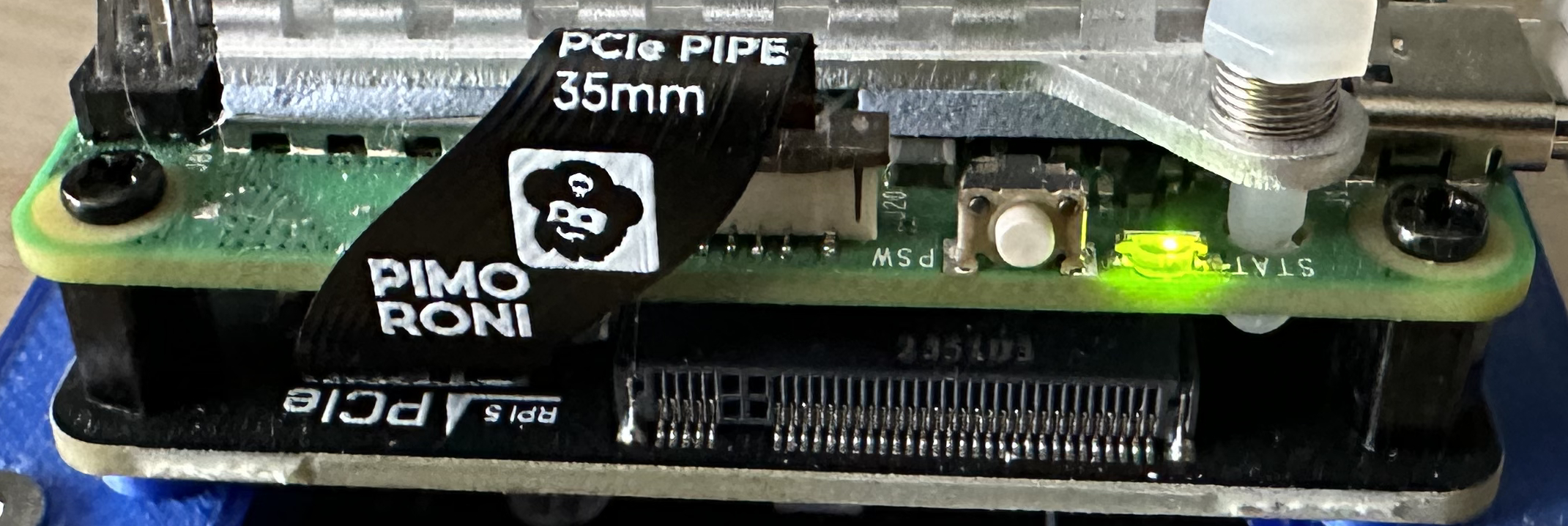
Assembly

Following the assembly guide was fairly painless. The most difficult step was to install the flat flex connector between the NVMe Base and the Raspberry Pi 5.

Configuration

The product page for the NVMe Base contains a good installation guide. This guide assumes that the SSD installed on the NVMe base is going to be used as the main boot drive for the system and that the OS etc. will be copied from existing bootable media. This is not the case for this installation.

System Update

As with all Pi setups, the first thing we should do is make sure that we have the most recent OS and software.

sudo apt get update -y
sudo apt get dist-upgrade -y
sudo reboot now

This should ensure that we have the latest and greatest deployed to the board.

Firmware Update and Setting the PCIe Mode

The first two steps are common to both the bootable scenario and this scenario. The firmware will need to be checked and if necessary updated and then experimental PCIe mode enabled.

Firstly, choose the boot ROM version and set this to the latest and reboot the system. The following command will configure the system to use the latest boot ROM.

sudo raspi-config nonint do_boot_rom E1 1
sudo reboot now

Further information on using the raspi-config tool in command mode can be found in the Raspi-Config documentation. Note however, that at the time of writing the documentation was slightly out of date as there was no mention of the need for the number 1 at the end of the command. This is required to answer No to the question about resetting the bootloader to the default configuration.

Next up, check the bootloader version and update this if necessary by using the rpi-eeprom-update command:

sudo rpi-eeprom-update

This generated the following output:

BOOTLOADER: up to date
   CURRENT: Fri 16 Feb 15:28:41 UTC 2024 (1708097321)
    LATEST: Fri 16 Feb 15:28:41 UTC 2024 (1708097321)
   RELEASE: latest (/lib/firmware/raspberrypi/bootloader-2712/latest)
            Use raspi-config to change the release.

PCIe Experimental Mode (Optional)

The last step is optional and turns on an experimental high speed feature, namely PCIe mode 3. Edit the /boot/firmware/config.txt file and add the following to the end of the file:

[all]
dtparam=pciex1_gen=3

This step is optional and without this entry the system will run in PCIe mode 2.

Reboot

So the boot loader is up to date, time for another reboot using the command sudo reboot now.

Mounting the Drive

We should now be at the point where the system has the correct configuration to allow access to the drive mounted to the NVMe Base. These drives should be in the /dev directory:

ls /dev/nv*

shows:

/dev/nvme0  /dev/nvme0n1

This looks good, as the drive shows up as the two devices. Now we need to put a file system on the drive, the following formats the drive using the ext4 file system:

sudo mkfs.ext4 /dev/nvme0n1 -L Data

For the 500GB ADATA drive supplied with the NVMe Base kit, this command generates the following:

mke2fs 1.47.0 (5-Feb-2023)
Discarding device blocks: done
Creating filesystem with 125026900 4k blocks and 31260672 inodes
Filesystem UUID: 008efe62-93f2-4875-bf52-5843953db8d0
Superblock backups stored on blocks:
	32768, 98304, 163840, 229376, 294912, 819200, 884736, 1605632, 2654208,
	4096000, 7962624, 11239424, 20480000, 23887872, 71663616, 78675968,
	102400000

Allocating group tables: done
Writing inode tables: done
Creating journal (262144 blocks): done
Writing superblocks and filesystem accounting information: done

Next up we need to mount the file system and make it accessible to the user. Assuming the default (current) user is pi and the user is in the group pi then the following commands will make the drive available to the current session:

sudo mkdir /mnt/nvme0
sudo chown -R pi:pi /mnt/nvme0
sudo mount /dev/nvme0n1 /mnt/nvme0

Firstly, we make the mount point for the partition and then ensure that the pi user has access to the mount point. Finally we mount the partition /dev/nvme0n1 as /mnt/nvme0. The availability of the drive can be checked with the df command, running:

df -h

should result in something like:

Filesystem      Size  Used Avail Use% Mounted on
udev            3.8G     0  3.8G   0% /dev
tmpfs           806M  5.2M  801M   1% /run
/dev/sda2       229G  1.8G  216G   1% /
tmpfs           4.0G     0  4.0G   0% /dev/shm
tmpfs           5.0M   48K  5.0M   1% /run/lock
/dev/sda1       510M   63M  448M  13% /boot/firmware
tmpfs           806M     0  806M   0% /run/user/1000
/dev/nvme0n1    469G   28K  445G   1% /mnt/nvme0

Access should now be checked by copying some files or creating a directory on the drive.

Mounting the Partition Automatically

The final step to take is to mount the partition and make the file system available as soon as the system boots. If the Raspberry Pi is rebooted now and the df -h command is run then something like the following is shown:

Filesystem      Size  Used Avail Use% Mounted on
udev            3.8G     0  3.8G   0% /dev
tmpfs           806M  5.2M  801M   1% /run
/dev/sda2       229G  1.8G  216G   1% /
tmpfs           4.0G     0  4.0G   0% /dev/shm
tmpfs           5.0M   48K  5.0M   1% /run/lock
/dev/sda1       510M   63M  448M  13% /boot/firmware
tmpfs           806M     0  806M   0% /run/user/1000

Note that the drive /mnt/nvme0 has not appeared in the list of file systems available. Executing ls /dev/nvm* shows the device is available but it has not been mounted.

The first step in mounting the drive automatically is to find the unique identified (UUID) for the device using the command:

sudo blkid /dev/nvme0n1

This resulted in the following output:

/dev/nvme0n1: LABEL="Data" UUID="008efe62-93f2-4875-bf52-5843953db8d0" BLOCK_SIZE="4096" TYPE="ext4"

Make a note of the UUID shown for your drive. The final step is to add this to the /etc/fstab file, so edit this file with the command:

sudo nano /etc/fstab

and add the following line to the end of the file:

UUID=008efe62-93f2-4875-bf52-5843953db8d0 /mnt/usb1 ext4 defaults,auto,users,rw,nofail,noatime 0 0

Remember to substitute the UUID for the drive on your system for the UUID above.

Time for one final reboot of the system and log on to the Raspberry Pi. Check the availability of the file system with the df -h command. The drive should now be available and accessible to the pi user as well as any users in the pi group.

Conclusion

The NVMe Base boards offer a way to add M-key NVMe SSD drives to the Raspberry Pi using PCIe gen 2 and even experimental access using PCIe gen 3. This results in high speed access to data stored on these drives as well as increased reliability over SD card boot devices.

The standard installation documentation is excellent but it assumes that the NVMe Base is going to host the OS as well as user data on the drive installed on the NVMe base. It also makes the assumption that the user will be using the Raspberry Pi desktop and not running in a headless situation.

Hopefully the above shows how to install the NVMe Base and SSD drive as a data storage only media with a second drive acting as the OS boot device.

In the next post we will look at taking the above steps and automating them to allow for reliable, repeated installations.

A few weeks ago I promised an update on my experience using the PCBWay and Round Tracks plugins for KiCAD.

Well the boards are back and I must say they are looking good.

Rounded Tracks Plugin

The rounded tracks plugin certainly gives the 1970s feel to the PCBs. The batch ordered had a gloss black finish and this made the rounded effect a little difficult to see, a matt finish may have looked better or maybe even a green PCB for that real 1970s vibe.

This plugin has seen a little more use since the first order and here are a few things I have picked up:

• Apply teardrops after using the plugin
• Keep the original PCB layout

Adding teardrops to the board really does give the retro feel to the board. I have found that rounding the tracks after adding teardrops can leave a disjoint connection between the track at the teardrop connection to the pad.

So here is a section of the board with the rounded tracks applied after the teardrops:

Rounded Track Applied After Teardrop

This shows that the track exits the corner of the teardrop which is not ideal. Next we have the same pad with the rounded tracks applied before the teardrops:

Rounded Track Applied Before Teardrop

The second case is certainly more aesthetically pleasing.

The plugin asks if you want to apply the changes to the current PCB or if it should create a copy. I went for the halfway house and applied the changes to the PCB, reviewed and ordered the boards and then reverted the changes. This worked well as the plugin ran in under a second and allowed the retention of the original design. It is always going to be easier to apply any changes to the PCB on a board with angular tracks than it is to apply the changes to a board with rounded tracks.

PCBWay Plugin

This plugin really made ordering the PCBs a dream. The only thing to remember is to login to your PCBWay account before attempting to use the plugin. If you do this the plugin will create and upload a ZIP file with the gerbers directly to your PCBWay account. This allows the plugin to set all of the parameters for board dimensions and layers all seamlessly.

Finished Boards

Here is a photo of the finished board connected to a Meadow F7 Micro board running a sok test:

Meadow and OLED Display

Conclusion

The Rounded Tracks plugin is only really of interest if you want the retro 1970 look and feel to the final PCB. The PCBWay plugin is really useful as it streamlines the ordering process and removes the need to manually create the gerber files and upload them to the PCBWay website.

A recent change to a PCB design has given the opportunity to try out a couple of KiCad plugins. The board is a simple one and is used to provide feedback when running network soak tests. The board is designed for the Meadow ecosystem and is a fairly simple design consisting of:

• SSD1306 OLED display
• Indicator LEDs
• Reset button
• Headers to connect the board to a Meadow board

The board has been tested and it works well. The changes doubled the number of LEDs and changed some of the components footprints.

Round Tracks

The concept behind Round Tracks is simple, take a PCB layout and give the tracks the feel of the 1970s. It does this by taking the layout and looking for any tracks that change direction. The plugin then takes these tracks and rounds the corners.

Applying this to the OLED PCBs gives the following output:

PCBWay Plug-in for KiCad

The next plugin is the PCBWay plugin. This should take the PCB layout and generate a zip file to upload to the PCBWay web site for manufacture. It appears to be really simple to use and starts an order for you and then uploads the files into the order.

Order submitted and now we just have to wait for the PCBs to arrive.

Conclusion

Manufacturing is complete and they are now on their way. There is going to be a small wait while the PCBs make their way from China to the UK and then we can see how the plugins faired.

Update to follow in a few weeks.

For the last year or so, the goto scope in the lab has been a Rigol MSO5104. This is a 100MHz, 4 channel scope with 16 digital channels. Connectivity options include USB and wired LAN. The LAN connection allows the scope to be controller via a web control panel which is great for interactive control from a host computer but is not much use for automation.

Enter pyvisa.

Hackaday Article

Hackaday published an article Grabbing Data From a Rigol Scope with Python in late November of 2023. It appears that I am not the only one looking to control a Rigol oscilloscope from a host computer.

The article discusses using pyvisa to communicate with a DHO900-series scope not a MSO5000-series scope, let’s see if the same commands will work with the MSO5104.

Communicating With The MSO5104

First up, try to connect to the scope over the LAN:

import pyvisa
visa = pyvisa.ResourceManager('@py')
scope = visa.open_resource('TCPIP::192.168.1.95::INSTR')

So that seemed to work, so let’s try to get the scope to identify itself:

scope.query('*IDN?')
'RIGOL TECHNOLOGIES,MSO5104,MS5A*********,00.01.03.03.00\n'

So far, so good, the * characters represent part of the devices serial number. Now let’s try a few commands to see if we can make the scope to do something:

scope.write(':SINGLE')
9

This changes the mode of the scope to single shot and the Single button turned on as if it had been pressed. The return value is the number of characters sent to the scope.

Conclusion

It appears that the original Hackaday article is going to be part of a series of articles as a follow-up article was published a few days later (see Scope GUI Made Easier). This could turn into something useful.

Recent work has involved reviewing some test environments for an IoT development board. The aim is to improve some of the components used for testing as well as adding new functionality. The requirements are:

• Provide an updated version of existing functionality
• Single board environment with all functionality deployed for quick testing
• Cluster distributing the test environment for load testing

The most cost effective way to do this is to use a number of Raspberry Pi single board computers. These boards are now becoming available in quantities after several years of limited availability.

The Problem

How to setup the environment in such a way that will allow a fresh environment to be created reliably.

Enter ansible.

Ping

First step, try to contact a board and this is where ping comes in. This command will verify that ansible can connect to a board. The following command will test the connection to each board:

ansible cluster -m ping -i hosts

This command requires a text file hosts containing the list of boards to the contacted. The file is simple and may only contact two lines:

[cluster]
node

In the above example, the file defines a group of machines to be contacted and this is named cluster and in this case the group contains only one machine and this is named node. The name cluster is also mentioned in the ansible command above.

Additional machines can also be named under the cluster entry by simply placing additional entries on a new line in the file.

So far this is nothing new and it is covered in the Ansible documentation.

What Happened

The first step was to use the Raspberry Pi Imager application to create a new image on a new SSD. Nothing complex:

• Raspberry Pi 64-bit Lite OS
• Set the machine name to be node
• Enable SSH
• Set the user name to clusteruser and give the user a secure password

The password was then stored on the local machine in an environment variable CLUSTER_PASSWORD to allow the scripts to be stored in source control without giving away any secrets.

Time to test the connection with the following command:

ansible cluster -m ping -i hosts --extra-vars "ansible_user=clusteruser ansible_password=$CLUSTER_PASSWORD"

Breaking this down, we want to ping all of the machines defined in the cluster group. The group is defined in the file hosts and we are going to log on to the machines with the user name clusteruser and with the password contained in the CLUSTER_PASSWORD environment variable.

Now running the above command results in the following:

node | SUCCESS => {
    "ansible_facts": {
        "discovered_interpreter_python": "/usr/bin/python3"
    },
    "changed": false,
    "ping": "pong"
}

Conclusion

A good start to the project, now on to something more complex, time to install and configure some software.

And I can’t believe I’ve missed Ansible for so long.

It may appear at the start of his story that this is an unhappy tale, but bear with it, there is a happy ending.

Having an oscilloscope when working with electronics is a must even for hobbyists. The amount of information you can gather about the behaviour of a circuit is invaluable. The daily workhorse here is the Rigol MSO5104 Mixed Signal Oscilloscope.

This scope is really a small computer and like all computers a regular check for firmware updates is always a good idea. A recent visit to the Rigol web site resulted in a new firmware version downloaded to the laptop.

Time to Install

Installation should be a quick process:

• Extract the files on the PC
• Copy the firmware file (.gel file) to a USB drive
• Connect the USB drive to the oscilloscope and select Local Update from the System menu

Following the process resulted in the update dialog being shown with a progress bar followed by instructions to restart the oscilloscope.

Power cycling the oscilloscope presented the expected Rigol logo along with a progress bar, so far, so good. The boot continued until just before the end of the process bar and then it stopped.

Wait a little while longer.

No movement after 5 minutes, time to power cycle. The same thing happened. Rinse and repeat, still no progress.

Time to call the local distributor.

Recovery

A call to the local Rigol distributor in the UK was in order. I found their technical support really good. In fact it was FAN-TAS-TIC. The solution turned out to be fairly simple.

• Power off the oscilloscope
• Turn the oscilloscope on again
• As the oscilloscope starts press the Single button repeatedly

Doing this would eventually show the Rigol logon on the screen with two options:

• Upgrade Firmware
• Recover Defaults

Selecting Recover Defaults took us through the recovery process and after a few minutes restoring the configuration and restarting the oscilloscope it was back up and running again.

Conclusion

Computers are all around us running in everything including the modern oscilloscope. Rigol has thoughtfully added a recovery mechanism into the firmware update process and so today all was not lost.

A call out to the UK distributors, the support was really, really good.

Time for some more experimentation with NuttX, today serial LCDs.

Serial LCDs

Small LCD displays can be found in many scientific instruments as they provide a simple way to display a small amount of information to the user. Typically these displays are 16×2 (2 lines of 16 characters) or 20×4 (4 lines of 20 characters) displays. The header to this article shows part of the output from a 20×4 display.

Communication with these displays is normally through a 4 or 8 bit interface when talking directly to the controller chip for the LCD. Using 4 or 8 data lines for communication with the LCD is a large burden on a small microcontroller. To overcome this, several vendors have produced a backpack that can be attached to the display. The backpack uses a smaller number of microcontroller lines for communication while still being able to talk to the LCD controller chip.

This post looks at using such and LCD and backpack with NuttX running on the Raspberry Pi Pico W.

NuttX Channel (Youtube)

A great place to start with NuttX is to have a look at the NuttX Channel on Youtube as there are a number of quick getting started tutorials covering a number of subject. In fact there is one covering a 16×2 LCD display which is similar to what will be used in this tutorial, with a small difference.

The video linked above covers a lot of what is needed to get 16×2 LCD up and running. There are some small changes that are needed as NuttX has moved on since the video was released.

Hardware

The major changes compared to the video above are:

• Microcontroller used will be the Raspberry Pi Pico W
• LCD display will be 20×4 display

The LCD display used here will be a larger physical display (20×4 instead of 16×2) but it will still use the same interface on the backpack, namely the PCF8574 GPIO expander. This uses I2C as a communication protocol so reduces the number of GPIO lines required from 8 to 2.

There are two I2C busses on the Pico W, I2C0 and I2C1 and in this case I2C1 will be the chosen interface. Something that caused some issues but more on that later.

For now we start with a base configuration with the LCd connected to GPIO6 and GPIO7 on the Pico W.

Configuring NuttX

Configuration followed much of the video linked above enabling the following:

• Enable I2C master and I2c1 in the System Type menu
• I2C Driver Support in the Device Drivers menu
• PCF8574 support through Device Drivers, Alphanumeric Drivers menus
• Segment LCD CODEC in the Library Routines menu
• Segment LCD Test in the Application Configuration, Examples menu

Time to build, deploy and run.

• make clean followed by make -j built the system
• The application was then deployed to the Pico W and board was reset
• The application can be run by connecting a terminal/serial application to the board an running the command slcd

Nothing appears on the display. Time to check the connections and break out the debugger.

Troubleshooting

Checking the connections showed that everything looked to be in order. The display was showing a faint pixel pattern which is typical of these displayed when they have been powered correctly but there is no communication. Double checking the I2C connections showed everything in theory was good.

Over to the software. Running through the configuration again and all looks good here. So lets try I2C0 instead of I2C1, quick change of the configuration in the software and moving some cables around and it works!

So lets go back to the I2C1 configuration, recompile and deploy to the board and it works. What!

It turns out that I had not moved the connections from I2C0 back to I2C1.

The default application was also only displaying 1 line of text. So let’s expand this to display 4 lines of text, namely:

• Hello
• Line1
• Line2
• Line3

Running the application gives only two line of text:

• Hello
• Line3

How odd.

Lets Read the Sources

After a few hours of tracing through the sources we find ourselves looking in the file rp2040_common_bringup.c where there is this block of code:

#ifdef CONFIG_LCD_BACKPACK
    /* slcd:0, i2c:0, rows=2, cols=16 */

    ret = board_lcd_backpack_init(0, 0, 2, 16);
    if (ret < 0)
    {
        syslog(LOG_ERR, "Failed to initialize PCF8574 LCD, error %d\n", ret);
        return ret;
        return ret;
    }
#endif

This suggests that the serial LCD test example is always configured to use a 16×2 LCD display on I2C0. This explains why we saw only two lines of output on the display and also why the code did not work on I2C1.

Changing ret = board_lcd_backpack_init(0, 0, 2, 16); to ret = board_lcd_backpack_init(0, 1, 4, 20); and recompiling generated the output we see at the top of this post.

Navigating to the System Type menu also allowed the I2C1 pins to be changed to 26 and 27 and the system continued to generate the expected results.

Conclusion

This piece of work took a little more time than expected and it would have been nice to have had the options within the configuration system to change the display and I2C parameters. As it stands at the moment using a 20×4 display requires changes to the OS source code. This is a trivial change but it does make merging / rebasing with later versions of the system a little more problematic.

A while ago I put together an emulator for the Small Scale Experimental Machine (SSEM), also known as the Manchester Baby. This was a basic console application allowing a program written for the Manchester Baby to be run in a console application on a modern computer. As things turned out, I now spend most of my time working in either C or C++. This has left me with a piece of code that is difficult to maintain as I have to relearn Python every time I want to make any improvements.

Time to rewrite the application in C++.

SSEM Simulator

The simulator provides a number of features:

• Assembler/compiler to take source files and generate the binary to be execution
• Console interface to control the execution of the application
• Simulated display of the registers and memory

More information about the Python version of the simulator can be found in this blog and on the Small Scale Experimental Machine web site with full source code available on GitHub.

Porting the Simulator

The aim of the initial port is to provide the same functionality of the original application with any changes necessary to provide additional robustness as we are undoubtedly going to be seeing pointers in the C++ port.

Where possible, the structure of the original Python code has been maintained to keep a 1:1 mapping with the original code and test suite. This will provide an easy way to validate the unit tests in the port against the original Python code. The original Python code was validated against David Sharps Java Simulator.

The long term aim of this port is to provide a way of running the application on a Raspberry Pi Pico connected to hardware which will emulate the original SSEM. The application on the Raspberry Pi Pico will target the NuttX RTOS. As we will see later, compiling and running on NuttX will present some interesting issues.

Initial Port

The first stage of the port is to reproduce the core functionality of the SSEM showing the application output in a console interface targeting C++ 17. The only real complication here is ensure the user interface and platform specific code are abstracted to keep as much functionality in common with a desktop and NuttX implementation as possible.

The original Python code and the C++ port can be found in the Manchester Baby GitHub repository. A quick check of the source code shows that the 1:1 mapping has been kept where possible. The only real significant difference between the two code bases is the separation of the unit tests from the class implementation. The Python code keeps the unit test code in the class definitions themselves, the C++ code implements the unit tests in their own files.

Memory Checks

The switch from Python to C++ brings a new danger, memory access issues and memory leaks.

One memory issue that we can address relatively easily is memory leaks. If we can abstract the core functionality into a self contained group of files then we can use valgrind to check for memory leaks. A small glitch with using valgrind is that the application is not available for Mac from the key repositories. There is an informal project on GitHub.

The issue of valgrind not running on the mach was resolved by putting together a Dockerfile containing common development tools. The memory check could then be run on the desktop using Docker.

Running the Emulator

The emulator can be run on both a desktop computer as well as a board running NuttX.

Run from the Desktop

Running the application on the desktop is the simplest way to test the emulator:

• Open a command console and change to the Desktop directory in the repository
• Build the emulator with the command make
• Run the emulator with the command ./ssem_main

Run on NuttX

Running on NuttX is a little more complex as we need to build the application and the operating system and then deploy the binary to a board. The processes of adding the SSEM application to a Raspberry Pi PicoW board has already been documented in the article Adding a User Application to NuttX. The first step is to follow the steps in the article to add the SSEM basic applicatiom.

The next stage is to copy the contents of the NuttX directory over the application directory created in the above article. The code should then be rebuilt with the command make clean && make -j. The application can now be deployed to the board.

Now we have the OS and the application deployed to the Raspberry Pi (or your board of choice) we can connect a serial adapter to the board and press the enter key twice. This will bring up the NuttX shell. Typing help should show the ssem application deployed to the board. Simply execute this by entering the command ssem.

Application Output

In both cases the emulator should run the hfr989.ssem application (the source for this can be found in the SSEMApps folder in the repository). Both the desktop and the NuttX versions of the emulator will run the SSEM application and will show the start and end state of the SSEM on the console / serial port. The first output will show the SSEM application loaded into the store lines:

NuttShell (NSH) NuttX-10.4.0
nsh> ssem
                   00000000001111111111222222222233
                   01234567890123456789012345678901
   0: 0x00000000 - 00000000000000000000000000000000 JMP 0            ; 0
   1: 0x48020000 - 01001000000000100000000000000000 LDN 18           ; 16402
   2: 0xc8020000 - 11001000000000100000000000000000 LDN 19           ; 16403
   3: 0x28010000 - 00101000000000010000000000000000 SUB 20           ; 32788
   4: 0x00030000 - 00000000000000110000000000000000 CMP              ; 49152
   5: 0xa8040000 - 10101000000001000000000000000000 JPR 21           ; 8213
   6: 0x68010000 - 01101000000000010000000000000000 SUB 22           ; 32790
   7: 0x18060000 - 00011000000001100000000000000000 STO 24           ; 24600
   8: 0x68020000 - 01101000000000100000000000000000 LDN 22           ; 16406
   9: 0xe8010000 - 11101000000000010000000000000000 SUB 23           ; 32791
  10: 0x28060000 - 00101000000001100000000000000000 STO 20           ; 24596
  11: 0x28020000 - 00101000000000100000000000000000 LDN 20           ; 16404
  12: 0x68060000 - 01101000000001100000000000000000 STO 22           ; 24598
  13: 0x18020000 - 00011000000000100000000000000000 LDN 24           ; 16408
  14: 0x00030000 - 00000000000000110000000000000000 CMP              ; 49152
  15: 0x98000000 - 10011000000000000000000000000000 JMP 25           ; 25
  16: 0x48000000 - 01001000000000000000000000000000 JMP 18           ; 18
  17: 0x00070000 - 00000000000001110000000000000000 HALT             ; 57344
  18: 0x00000000 - 00000000000000000000000000000000 JMP 0            ; 0
  19: 0xc43fffff - 11000100001111111111111111111111 HALT             ; -989
  20: 0x3bc00000 - 00111011110000000000000000000000 JMP 28           ; 988
  21: 0xbfffffff - 10111111111111111111111111111111 HALT             ; -3
  22: 0x243fffff - 00100100001111111111111111111111 HALT             ; -988
  23: 0x80000000 - 10000000000000000000000000000000 JMP 1            ; 1
  24: 0x00000000 - 00000000000000000000000000000000 JMP 0            ; 0
  25: 0x08000000 - 00001000000000000000000000000000 JMP 16           ; 16
  26: 0x00000000 - 00000000000000000000000000000000 JMP 0            ; 0
  27: 0x00000000 - 00000000000000000000000000000000 JMP 0            ; 0
  28: 0x00000000 - 00000000000000000000000000000000 JMP 0            ; 0
  29: 0x00000000 - 00000000000000000000000000000000 JMP 0            ; 0
  30: 0x00000000 - 00000000000000000000000000000000 JMP 0            ; 0
  31: 0x00000000 - 00000000000000000000000000000000 JMP 0            ; 0

Reading from left to right, the above output shows the following:

• Store line number (i.e. the memory address) 0:, 1: etc.
• The hexadecimal representation of the store line contents.
• Binary representation of the store line contents
• Disassembled representation of the store line contents JMP 0 etc.
• Decimal representation of the store line contents

It must be remembered when reading the above that the least significant bit is at the left of the word and the most significant bit is to the right. This is honoured with the hexadecimal and binary components of the above output. The decimal value to the right should be read in the usual way for a base 10 number.

After a short time the contents of the store lines at the end of the run will be displayed:

Program execution complete.
                   00000000001111111111222222222233
                   01234567890123456789012345678901
   0: 0x00000000 - 00000000000000000000000000000000 JMP 0            ; 0
   1: 0x48020000 - 01001000000000100000000000000000 LDN 18           ; 16402
   2: 0xc8020000 - 11001000000000100000000000000000 LDN 19           ; 16403
   3: 0x28010000 - 00101000000000010000000000000000 SUB 20           ; 32788
   4: 0x00030000 - 00000000000000110000000000000000 CMP              ; 49152
   5: 0xa8040000 - 10101000000001000000000000000000 JPR 21           ; 8213
   6: 0x68010000 - 01101000000000010000000000000000 SUB 22           ; 32790
   7: 0x18060000 - 00011000000001100000000000000000 STO 24           ; 24600
   8: 0x68020000 - 01101000000000100000000000000000 LDN 22           ; 16406
   9: 0xe8010000 - 11101000000000010000000000000000 SUB 23           ; 32791
  10: 0x28060000 - 00101000000001100000000000000000 STO 20           ; 24596
  11: 0x28020000 - 00101000000000100000000000000000 LDN 20           ; 16404
  12: 0x68060000 - 01101000000001100000000000000000 STO 22           ; 24598
  13: 0x18020000 - 00011000000000100000000000000000 LDN 24           ; 16408
  14: 0x00030000 - 00000000000000110000000000000000 CMP              ; 49152
  15: 0x98000000 - 10011000000000000000000000000000 JMP 25           ; 25
  16: 0x48000000 - 01001000000000000000000000000000 JMP 18           ; 18
  17: 0x00070000 - 00000000000001110000000000000000 HALT             ; 57344
  18: 0x00000000 - 00000000000000000000000000000000 JMP 0            ; 0
  19: 0xc43fffff - 11000100001111111111111111111111 HALT             ; -989
  20: 0x54000000 - 01010100000000000000000000000000 JMP 10           ; 42
  21: 0xbfffffff - 10111111111111111111111111111111 HALT             ; -3
  22: 0x6bffffff - 01101011111111111111111111111111 HALT             ; -42
  23: 0x80000000 - 10000000000000000000000000000000 JMP 1            ; 1
  24: 0x00000000 - 00000000000000000000000000000000 JMP 0            ; 0
  25: 0x08000000 - 00001000000000000000000000000000 JMP 16           ; 16
  26: 0x00000000 - 00000000000000000000000000000000 JMP 0            ; 0
  27: 0x00000000 - 00000000000000000000000000000000 JMP 0            ; 0
  28: 0x00000000 - 00000000000000000000000000000000 JMP 0            ; 0
  29: 0x00000000 - 00000000000000000000000000000000 JMP 0            ; 0
  30: 0x00000000 - 00000000000000000000000000000000 JMP 0            ; 0
  31: 0x00000000 - 00000000000000000000000000000000 JMP 0            ; 0
Executed 21387 instructions in 30000000 nanoseconds

The original SSEM ran at about 700 instructions per second, modern PCs and even RP2040 processors are running the application much faster.

Conclusion

Even small boards (such as the Raspberry Pi Pico) running relatively low power processors can now emulate the Manchester Baby running application intended for the SSEM many times faster that the original hardware. The hfr989.ssem application would have run in about 30 seconds in 1948, today we can run this in an emulator in less that 30ms.

One feature that I want to add to my current project is to add a small file system with files that have been built into the system at compile time. These files would then be available to the application at run time. Let’s look at how we can do can do this with NuttX.

This tutorial assumes that you have NuttX cloned and ready to build, if not then you can find out how to do this in the first article in this series.

Adding SmartFS to the Build

NuttX has a built in configuration for the PicoW with SmartFS already configured. The first thing we need to do is to start with a clean system and then configure the build to include NSH and the flash file system. Start by changing to the NuttX source directory and then executing the following commands:

make distclean
./tools/configure.sh -l raspberrypi-pico-w:nsh-flash

Now we have the system configured we can build the OS and applications by executing the following command:

make -j

This should take a minute or so on a modern machine. Now we can deploy the system to the PicoW either by using openocd or by dragging the uf2 file onto the PicoW drive. Now connect to the PicoW using a serial application and type help to show the menu of commands. You should see something like the following:

SmartFS Builtin Apps

We can check to see if the SmartFS is available checking the contents of the /dev directory with the command ls /dev. This should result in something like the following if SmartFS has been enabled correctly:

Device Directory Listing

We can mount the file system using the command mount -t smartfs /dev/smart0 /data and then check the contents of the /data directory and we should find one file in the directory, test. Checking the contents of the file with the command cat /data/test should find that it contains a single ine of text which should be Hello, world!.

So far, so good, we have built the system and proven that it contains the default file and correct contents.

Adding a New File to the System Image

The next piece of the puzzle is to work out how to add new files to the file system. This took a few hours to figure out, but here goes…

The first attempt lead me searching for RP2040_FLASH_FILE_SYSTEM in the source tree (ripgrep is a great tool for doing this). This lead to a number of possible files. Maybe we can narrow the search down a little.

Second attempt, let’s have a look for Hello, world!. This resulted in a smaller number of files leading to the file arch/arm/src/rp2040/rp2040_flash_initialize.S. This file is well documented and shows how to set up the SmartFS file system and at the end of the file it shows how to create an entry for the file we see when we list the mounted directory. Scrolling down to the end of the fie we find the following:

    sector      3, dir
    file_entry  0777, 4, 0, "test"

    sector      4, file, used=14
    .ascii      "Hello, world!\n"

    .balign     4096, 0xff
    .global     rp2040_smart_flash_end
rp2040_smart_flash_end:

This looks remarkably familiar. So what happens if we change the above to look like this:

    sector      3, dir
    file_entry  0777, 4, 0, "test"
    file_entry  0777, 5, 0, "test2"

    sector      4, file, used=14
    .ascii      "Hello, world!\n"

    sector      5, file, used=14
    .ascii      "Testing 1 2 3\n"

    .balign     4096, 0xff
    .global     rp2040_smart_flash_end
rp2040_smart_flash_end:

Building the system, deploying the code and executing the following commands:

mount -t smartfs /dev/smart0 /data
cd /data
ls

results in the following:

New file added to SmartFS

If we execute the command cat test2 we are rewarded with the output Testing 1 2 3.

Further testing shows that the file system survives through a reset. We can do the following:

• echo “My test” > test3
• rm test
• reboot

These commands should remove the file test, create a new file test3 and then reboot the system. Checking the file system contents shows that the system persists the changes through a reset.

Conclusion

This experiment was a partial success. A simple file system has been made available to an application and the file system survives a reset. One issue remains, adding new files is a little complex. It also requires changes to the NuttX source tree outside of the applications folder. This could result in changes being lost when a new version of NuttX is released.

There could be a solution, ROMFS, stay tuned for the next episode.

In the previous post, we managed to get GDB working with NuttX running on the Raspberry Pi PicoW. In this post we will look at using VSCode to debug NuttX.

For a large part of this post it was case of following Shawn Hymels guide Raspberry Pi Pico and RP2040 – C/C++ Part 2 Debugging with VS Code. This is an excellent guide and I recommend using it as a companion to this post.

We will start with the assumption that you have followed the previous post in this series and have a working NuttX build for the Raspberry Pi PicoW. We will also assume that you have a working VSCode installation with the Cortex-Debug extension installed.

Configuration Files

We will need to create (or modify) three configuration files to allow VSCode to debug NuttX.

• launch.json
• tasks.json
• settings.json

In the first article of this series we created the directory NuttX-PicoW to hold the apps and nuttx folders holding out NuttX code. This directory is the project directory or in VS Code parlance, the workspaceFolder. The workspaceFolder should also contain the Raspberry Pi PicoW SDK and the Raspberry Pi specific version of openocd.

We now add a .vscode directory to the workspaceFolder. This directory will hold the three configuration files listed above.

Start by opening VS Code and opening the workspaceFolder. This should show the four folders already in the workspaceFolder. Now create a .vscode directory in the workspaceFolder if it does not already exist.

setting.json

Only one entry is required in the settings.json file and this is the location of the openocd executable. If you have followed these posts so far this will be in the openocd/src folder. Create a setting.json file in the .vscode folder and add the following to the file.

{
    "cortex-debug.openocdPath": "${workspaceFolder}/openocd/src/openocd"
}

Note that the name of the executable may vary depending upon your operating system this post is being written from a MacOS perspective.

tasks.json

The tasks.json file holds the entry that will be used to build NuttX prior to deployment. In Shawns document the projects being worked on use the cmake system. We need to modify this to build NuttX using make. We want VS Code to use the command make -C ${workspaceFolder}/nuttx -j to build NuttX. The build task below will create a task Build NuttX to do just this:

{
    "version": "2.0.0",
    "tasks": [
        {
          "label": "Build NuttX",
          "type": "cppbuild",
          "command": "make",
          "args": [
            "-C",
            "${workspaceFolder}/nuttx",
            "-j"
          ]
        }
      ]  
}

launch.json

Of the three files we are creating, the launch.json file is the most complex. Much of the file remains the same as that presented by Shawn but there are some differences. The file used here looks like this:

{
    "version": "0.2.0",
    "configurations": [
        {
            "name": "Pico Debug",
            "cwd": "${workspaceRoot}",
            "executable": "${workspaceFolder}/nuttx/nuttx.elf",
            "request": "launch",
            "type": "cortex-debug",
            "servertype": "openocd",
            "gdbPath" : "arm-none-eabi-gdb",
            "device": "RP2040",
            "configFiles": [
                "interface/cmsis-dap.cfg",
                "target/rp2040.cfg"
            ],
            "svdFile": "${workspaceFolder}/pico-sdk/src/rp2040/hardware_regs/rp2040.svd",
            "runToEntryPoint": "__start",
            "searchDir": ["${workspaceFolder}/openocd/tcl"],
            "openOCDLaunchCommands": ["adapter speed 5000"],
            "preLaunchTask": "Build NuttX"
        }
    ]
}

The following items are the ones that need to be changed:

“executable”: “${workspaceFolder}/nuttx/nuttx.elf”

This is the path to the executable that will be created by the build system. In this cse it is the NuttX ELF file. This may need to be changed to “executable”: “${workspaceFolder}/nuttx/nuttx” depending upon the output of the build system, this may simply be nuttx.

“configFiles”

The recent versions of the picoprobe software use a different interface to talk to the picoprobe. For versions 1.01 and above of the picoprobe software this interface changed from picoprobe.cfg to cmsis-dap.cfg.

“svdFile”: “${workspaceFolder}/pico-sdk/src/rp2040/hardware_regs/rp2040.svd”

We have a version of the Pico SDK specifically for our build requirements and so for this reason the location of the file is changed to reference the workspaceFolder rather than the global PICO_SDK_PATH environment variable.

“runToEntryPoint”: “__start”

This entry replaces the “runToMain”: true entry. Unlike convention C/C++ applications, NuttX does not have a main method. Having the runToMain entry generates an error stating that main cannot be found and stops at the first executable statement in our code, namely in __start. Replacing runToMain with runToEntryPoint achieves the same thing but does not generate the error.

Doing this also removes the need to have the postRestartCommands specified.

“searchDir”: [“${workspaceFolder}/openocd/tcl”]

This entry is used by openocd to look for the interface and target configuration files specified in the configFiles entry.

“openOCDLaunchCommands”: [“adapter speed 5000”]

These commands are executed by openocd when it starts. The change to the adapter speed is required and is documented in Getting Started with Raspberry Pi Pico documentation from the Raspberry Pi Foundation.

“preLaunchTask”: “Build NuttX”

The final entry tells Cortex-Debug how to build NuttX. It references the task we previously defined in the tasks.json file.

Testing

Testing this should simply be a case of saving all of the files above and pressing F5 in VS Code. If the changes have been successful then VS Code will first try to build NuttX in a Terminal window and it will then deploy NuttX to the Pico board and start the debugger. VS Code should look something like this (click on image for full view):

Debugging PicoW with VSCode

The inclusion of the SVD file allows us to examine the PicoW peripheral registers as well as the core registers:

PicoW Peripheral Registers in VSCode	Pico Cortex Registers in VSCode

Conclusion

GDB is a great debugger but it is often more convenient to use an IDE to debug your code. VS Code with the Cortex-Debug extension allow visual debugging of NuttX with a few nice additional features thrown in:

• Easily viewed call stacks for both cores.
• The SVD file allows the peripheral registers to be viewed through VS Code

We should also note that the use of VS Code resolved the issues noted at the end of the previous post as Cortex-Debug is able to deploy a binary using the picoprobe without resorting to the UF2 method of deployment. This results in a seamless build, deploy and debug process.

We have two debug options and it is now down to personal preferences as to which one to use.